Derive And Translate Trajectory Calculations Into Code

Task: Derive And Translate Trajectory Calculations Into Code

To ease the work put on the drivers, we wanted to have the robot automatically shoot into the goal. This would improve cycle times by allowing the drivers, theoretically, to shoot from any location on the field, and avoids the need for the robot to be in a specific location each time it shoots, eliminating the time needed to drive and align to a location after intaking disks.

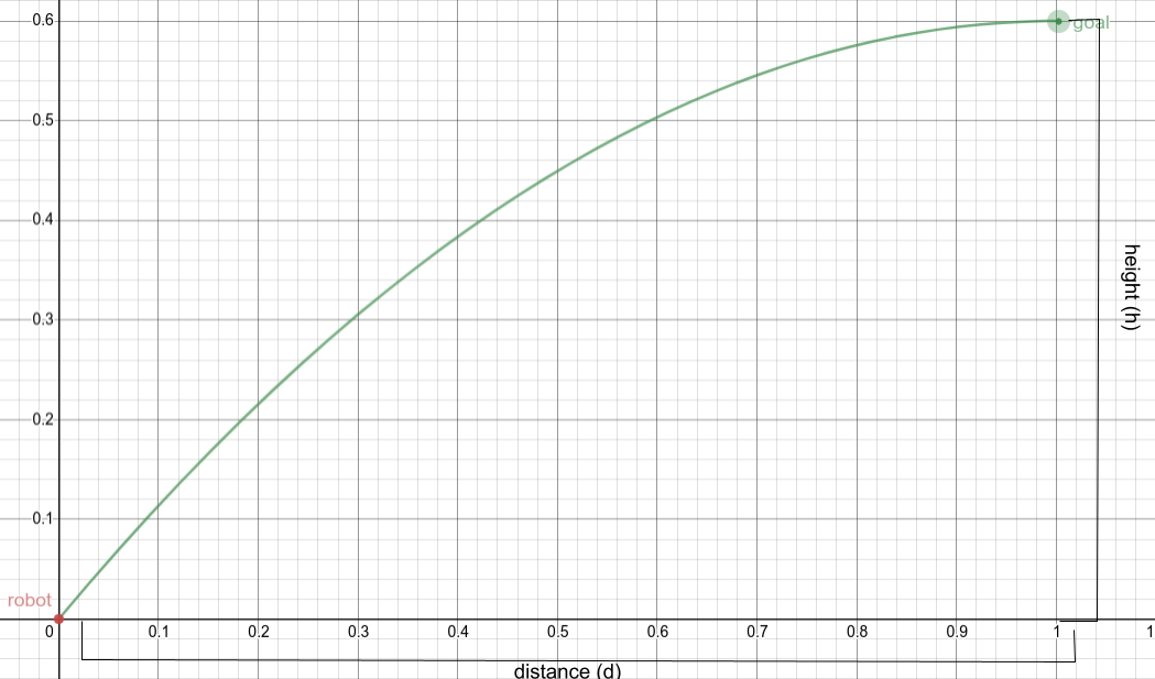
To be able to have the robot automatically shoot, we needed to derive the equations necessary to get the desired \(\theta\) (angle of launch) and \(v_0\) (initial velocity) values. This would be done given a few constants, the height of travel (the height of the goal - the height of the robot, which we will call \(h\)), the distance between the robot and the goal (which we will call \(d\)), and of course acceleration due to gravity, \(g\) (approximately \(9.8 \frac{m}{s^2}\)). \(d\) would be given through either a distance sensor, or using vuforia. Either way, we can assume this value is constant for a specific trajectory. Given these values, we can calculate \(\theta\) and \(v_0 \).

However, without any constraints multiple solutions exist, which is why we created a constraint to both limit the number of solutions and reduce the margin of error of the disk's trajectory near the goal. We added the constraint the disk should reach the summit (or apex) of its trajectory at the point at which it enters the goal, or that it's vertical velocity component is \(0\) when it enters the goal. This way there exists only one \(\theta\) and \(v_0\) that can launch the disk into the goal.

We start by outlining the basic kinematic equations which model any object's trajectory under constant acceleration: \[\displaylines{v = v_0 + at \\ v^2 = v_0^2 + 2a\Delta x \\ \Delta x = x_0 + v_0t + \frac{1}{2}at^2}\]

When plugging in the constants, considering the constraints mentioned before into these equations, accounting for both the horizontal and vertical components of motion, we get the following equations: \[\displaylines{0 = v_0sin(\theta) - gt \\ 0^2 = (v_0sin(\theta))^2 - 2gh \\ d = v_0cos(\theta)t}\] The first equation comes from using the first kinematic equation in the vertical component of motion, as the final velocity of the disk should be \(0\) according to the constraints, \(-g\) acts as the acceleration, and \(v_0sin(\theta)\) represents the vertical component of the launch velocity. The second equation comes from using the second kinematics equation again in the vertical component of motion, and again according to the constraints, \(-g\) acts as the acceleration, \(h\) represents the distance travelled vertically by the disk, and \(v_0sin(\theta)\) represents the vertical component of the launch velocity. The last equation comes from applying the third kinematics equation in the horizontal component of motion, with \(d\) being the distance travelled by the disk horizontally, \(v_0cos(\theta)\) representing the horizontal component of the launch velocity, and \(t\) representing the flight time of the disk.

Solving for \(v_0sin(\theta)\) in the first equation and substituting this for \(v_0sin(\theta)\) in the second equation gives: \[\displaylines{v_0sin(\theta) = gt \\ 0^2 = (gt)^2 - 2gh, t = \sqrt{\frac{2h}{g}}}\] Now that an equation is derived for \(t\) in terms of known values, we can treat t as a constant/known value and continue.

Using pythagorean theorem, we can find the initial velocity of launch \(v_0\). \(v_0cos(\theta)\) and \(v_0sin(\theta)\) can be treated as two legs of a right triangle, with \(v_0\) being the hypotenuse. Therefore \(v_0 = \sqrt{(v_0cos(\theta))^2 + (v_0sin(\theta))^2}\), so: \[\displaylines{v_0sin(\theta) = gt \\ v_0cos(\theta) = \frac{d}{t} \\ v_0 = \sqrt{(gt)^2 + {\left( \frac{d}{t}\right) ^2}}}\]

Now that \(v_0\) has been solved for, \(\theta\) can be solved for using \(sin^{-1}\) like so: \[\displaylines{\theta = sin^{-1}\left( \frac{v_0sin(\theta)}{v_0} \right) = sin^{-1}\left( \frac{gt}{v}\right) }\]

In order to be practically useful, the \(v_0\) previously found must be converted into a ticks per second value for the flywheel motor to maintain in order to have a tangential velocity equal to \(v_0\). In other words, a linear velocity must be converted into an angular velocity. This can be done using the following equation, where \(v\) = tangential velocity, \(\omega\) = angular velocity, and \(r\) = radius. \[\displaylines{v = \omega r, \omega = \frac{v}{r} \\ }\] The radius of the flywheel \(r\) can be considered a constant, and \(v\) is substituted for the \(v_0\) solved for previously.

However, this value for \(\omega\) is in \(\frac{radians}{second}\), but has to be converted to \(\frac{encoder \space ticks}{second}\) to be usable. This can be done easily with the following expression: \[\displaylines{\frac{\omega \space radians}{1 \space second} \cdot \frac{1 \space revolution}{2\pi \space radians} \cdot \frac{20 \space encoder \space ticks \space per \space revolution}{1 \space revolution} \cdot \frac{3 \space encoder \space ticks}{1 \space encoder \space tick}}\] The last \(\frac{3 \space encoder \space ticks}{1 \space encoder \space tick}\) comes from a \(3:1\) gearbox placed on top of the flywheel motor.

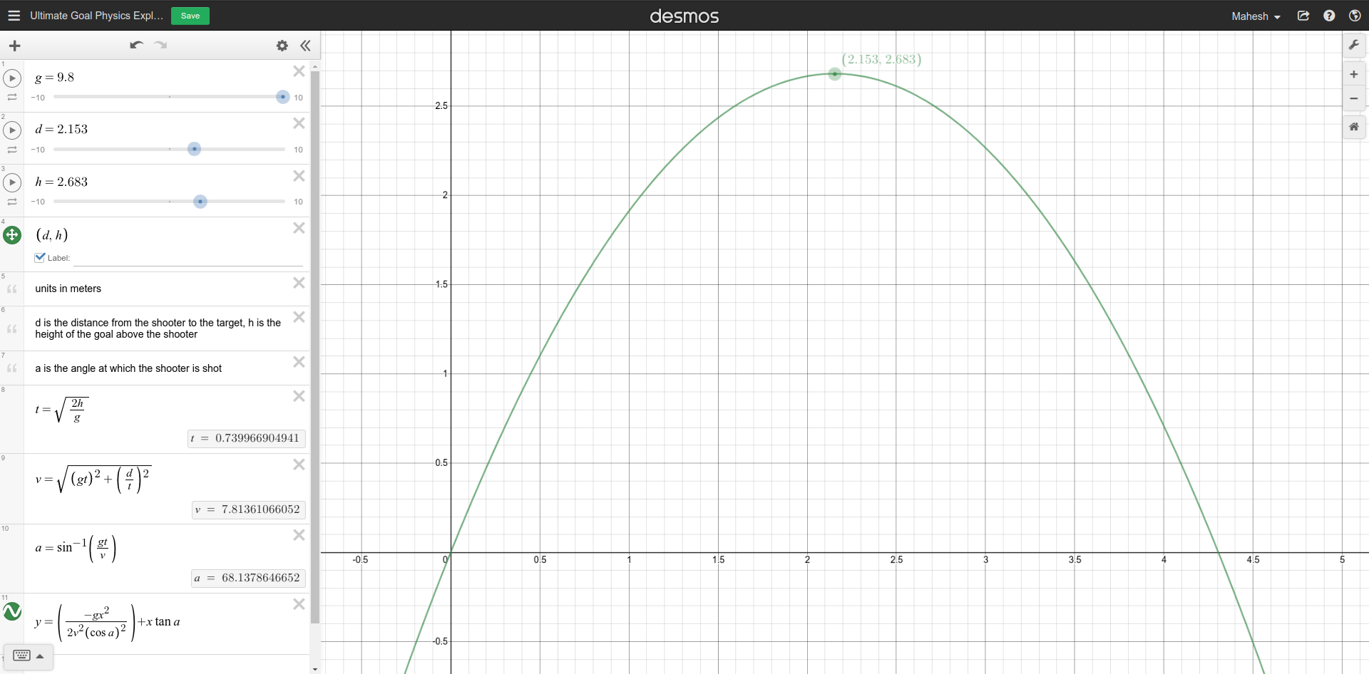
To sanity check these calculations and confirm that they would indeed work, we used a desmos graph, originally created by Jose and later modified with the updated calculations, to take in the constants used previously and graph out the parabola of a disk's trajectory. The link to the desmos is https://www.desmos.com/calculator/zuoa50ilmz, and the image below shows an example of a disk's trajectory.

To translate these calculations into code, we created a class named TrajectoryCalculator, originally created by Shawn and later refactored to include the updated calculations. To hold both an angle and velocity solution, we created a simple class, or struct, named TrajectorySolution. Both classes are shown below.

public class TrajectoryCalculator {
        private double distance;

        public TrajectoryCalculator(double distance) {
            this.distance = distance;
        }
    
        public TrajectorySolution getTrajectorySolution() {
            // vertical distance in meters the disk has to travel
            double travelHeight = Constants.GOAL_HEIGHT - Constants.LAUNCH_HEIGHT;
            // time the disk is in air in seconds
            double flightTime = Math.sqrt((2 * travelHeight) / Constants.GRAVITY);
    
            // using pythagorean theorem to find magnitude of muzzle velocity (in m/s)
            double horizontalVelocity = distance / flightTime;
            double verticalVelocity = Constants.GRAVITY * flightTime;
            double velocity = Math.sqrt(Math.pow(horizontalVelocity, 2) + Math.pow(verticalVelocity, 2));
    
            // converting tangential velocity in m/s into angular velocity in ticks/s
            double angularVelocity = velocity / Constants.FLYWHEEL_RADIUS; // angular velocity in radians/s
            angularVelocity *= (Constants.ENCODER_TICKS_PER_REVOLUTION * Constants.TURRET_GEAR_RATIO) / (2 * Math.PI); // angular velocity in ticks/s
    
            double theta = Math.asin((Constants.GRAVITY * flightTime) / velocity);
            return new TrajectorySolution(angularVelocity, theta);
        }
    }
    

public class TrajectorySolution {
    private double angularVelocity;
    private double theta;

    public TrajectorySolution(double angularVelocity, double theta) {
        this.angularVelocity = angularVelocity;
        this.theta = theta;
    }

    public double getAngularVelocity() {
        return angularVelocity;
    }

    public double getTheta() {
        return theta;
    }
}

Next Steps:

The next step is to use PID control to maintain target velocities and angles. The calculated angular velocity \(\omega\) can be set as the target value of a PID controller in order to accurately have the flywheel motor hold the required \(\omega\). The target angle of launch above the horizontal \(\theta\) can easily be converted into encoder ticks, which can be used again in conjunction with a PID controller to have the elbow motor maintain a position.

Another important step is to of course figure out how \(d\) would be measured. Experimentation with vuforia and/or distance sensors is necessary to have a required input to the trajectory calculations. From there, it's a matter of fine tuning values and correcting any errors in the system.