Deriving Inverse Kinematics For The Drivetrain

By Mahesh, Cooper, and Ben

Task: Derive Inverse Kinematics For The Drivetrain

Due to having an unconventential drivetrain consisting of two differental wheels and a third swerve wheel, it is crucial that we derive the inverse wheel kinematics early on. These inverse kinematics would convert a desired linear and angular velocity of the robot to individual wheel velocities and an angle for the back swerve wheel. Not only would these inverse kinematics be used during Tele-Op to control the robot through joystick movements, but it will be useful for getting the robot to travel at a desired forward velocity and turning rate for autonomous path following. Either way, deriving basic inverse kinematics for the drivetrain is a necessity prerequisite for most future programming endeavors.

More concretely, the problem consists of the following:
Given a desired linear velocity \(v\) and turning rate/angular velocity \(\omega\), compute the required wheel velocities \(v_l\), \(v_r\), and \(v_s\), as well as the required swerve wheel angle \(\theta\) to produce the given inputs. We will define \(v_l\) as the velocity of the left wheel, \(v_r\) as the velocity of the right wheel, and \(v_s\) as the velocity of the swerve wheel.

To begin, we can consider the problem from the perspective of the robot turning with a given turning radius \(r\) with tangent velocity \(v\). From the equation \(v = \omega r\), we can conclude that \(r = \frac{v}{\omega}\). Notice that this means when \(\omega = 0\), the radius blows up to infinity. Intuitively, this makes sense, as traveling in a straight line (\(\omega = 0\)) is equivalent to turning with an infinite radius.

The main equation used for inverse wheel kinematics is:

\[\displaylines{\vec{v_b} = \vec{v_a} + \vec{\omega_a} \times \vec{r}}\]

Where \(\vec{v_b}\) is the velocity at a point B, \(\vec{v_a}\) is the velocity vector at a point A, \(\vec{\omega_a}\) is the angular velocity vector at A, and \(\vec{r}\) is the distance vector pointing from A to B. The angular velocity vector will point out from the 2-D plane of the robot in the third, \(\hat{k}\), axis (provable using the right-hand rule).

But why exactly does this equation work? What connection does the cross product have with deriving inverse kinematics? In the following section, the above equation will be proven. See section 1.1 to skip past the proof.

To understand the equation, we start by considering a point A rotating around aother point B with turn radius vector \(\hat{r}\) and tangent velocity \(\vec{v}\).

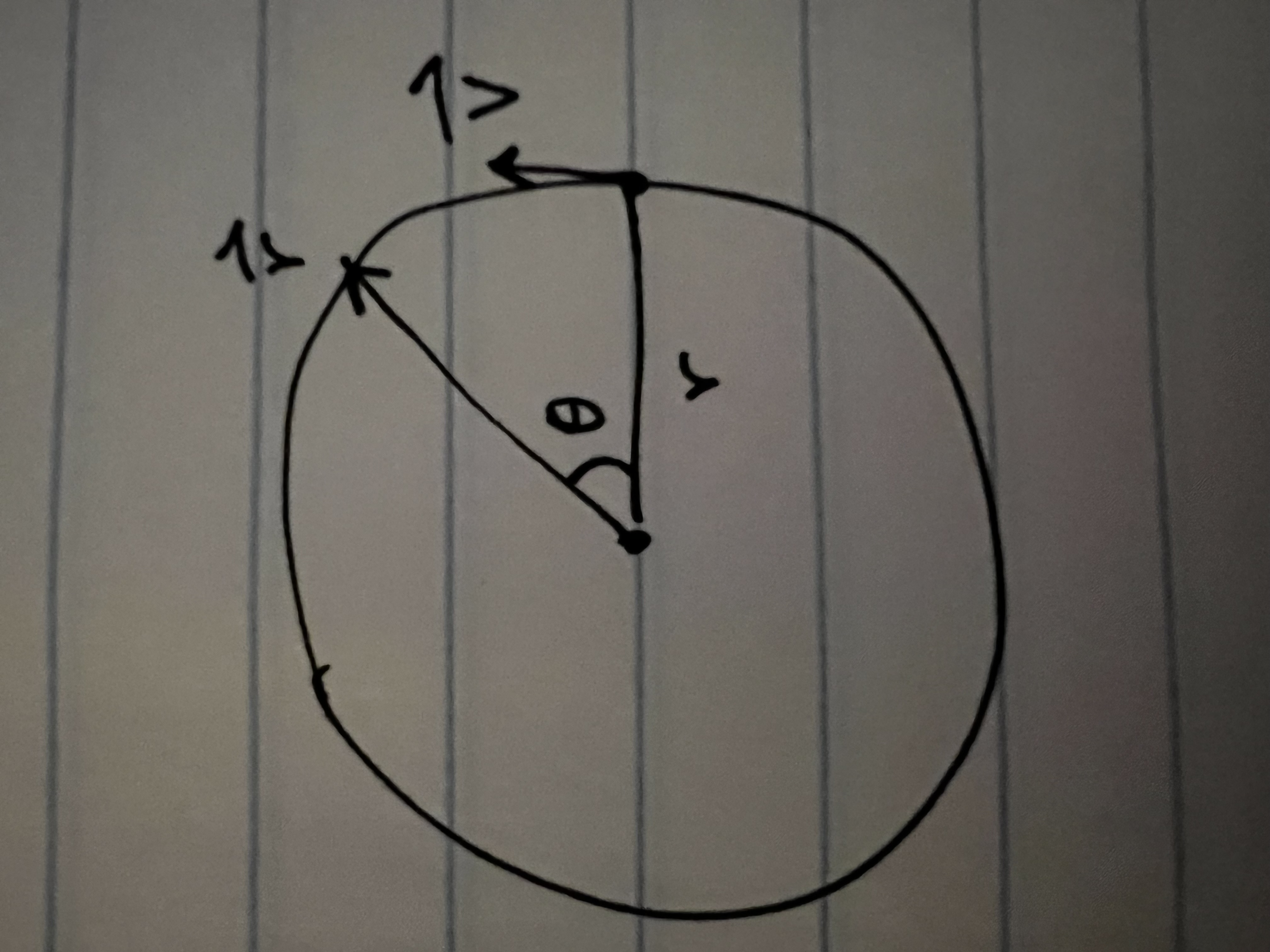
For an angle \(\theta\) around the x-axis, the position vector \(\vec{s}\) can be defined as the following:

\[\displaylines{\vec{s} = r(\hat{i}\cos\theta + \hat{j}\sin\theta) }\]

by splitting the radius vector into its components and recombining them.

To arrive at a desired equation for \(\vec{v}\), we will have to differentiate \(\vec{r}\) with respect to time. By the chain rule:

\[\displaylines{\vec{v} = \frac{d\vec{s}}{dt} = \frac{d\vec{s}}{d\theta} \cdot \frac{d\theta}{dt}}\]

The appropriate equations for \(\frac{d\vec{s}}{d\theta}\) and \(\frac{d\theta}{dt}\) can then be multiplied to produce the desired \(\vec{v}\):

\[\displaylines{\frac{d\vec{s}}{d\theta} = \frac{d}{d\theta} \vec{s} = \frac{d}{d\theta} r(\hat{i}\cos\theta + \hat{j}\sin\theta) = r(-\hat{i}sin\theta + \hat{j}cos\theta) \\ \frac{d\theta}{dt} = \omega \\ \vec{v} = \frac{d\vec{s}}{dt} = \frac{d\vec{s}}{d\theta} \cdot \frac{d\theta}{dt} = r(-\hat{i}sin\theta + \hat{j}cos\theta) \cdot \omega \mathbf{= \omega r(-\hat{i}sin\theta + \hat{j}cos\theta)} }\]

Now that we have an equation for \(\vec{v}\) defined in terms of \(\omega\), \(r\), and \(\theta\), if we can derive the same formula using \(\vec{\omega} \times \vec{r}\), we will have proved that \(\vec{v} = \frac{d\vec{s}}{dt} = \vec{\omega} \times \vec{r}\)

To begin, we will define the following \(\vec{\omega}\) and \(\vec{r}\):

\[\displaylines{ \vec{\omega} = \omega \hat{k} = \begin{bmatrix}0 & 0 & \omega\end{bmatrix} \\ \vec{r} = r(\hat{i}cos\theta + \hat{j}sin\theta) = \hat{i}rcos\theta + \hat{j}rsin\theta = \begin{bmatrix}rcos\theta & rsin\theta & 0\end{bmatrix} }\]

Then, by the definition of a cross product:

\[\displaylines{ \vec{\omega} \times \vec{r} = \begin{vmatrix} \hat{i} & \hat{j} & \hat{k} \\ 0 & 0 & \omega \\ rcos\theta & rsin\theta & 0 \end{vmatrix} \\ = \hat{i}\begin{vmatrix} 0 & \omega \\ rsin\theta & 0\end{vmatrix} - \hat{j}\begin{vmatrix} 0 & \omega \\ rcos\theta & 0\end{vmatrix} + \hat{k}\begin{vmatrix} 0 & 0 \\ rcos\theta & rsin\theta\end{vmatrix} \\ = \hat{i}(-\omega rsin\theta) - \hat{j}(-\omega rcos\theta) + \hat{k}(0) \\ \mathbf{= \omega r(-\hat{i}sin\theta + \hat{j}cos\theta)}}\]

Since the same resulting equation, \(\omega r(-\hat{i}sin\theta + \hat{j}cos\theta)\), is produced from evaluating the cross product of \(\vec{\omega}\) and \(\vec{r}\) and by evaluating \(\frac{d\vec{s}}{dt}\), we can conclude that \(\vec{v} = \vec{\omega} \times \vec{r}\)

1.1

Based on the constants defined and geometry defined in the image below:

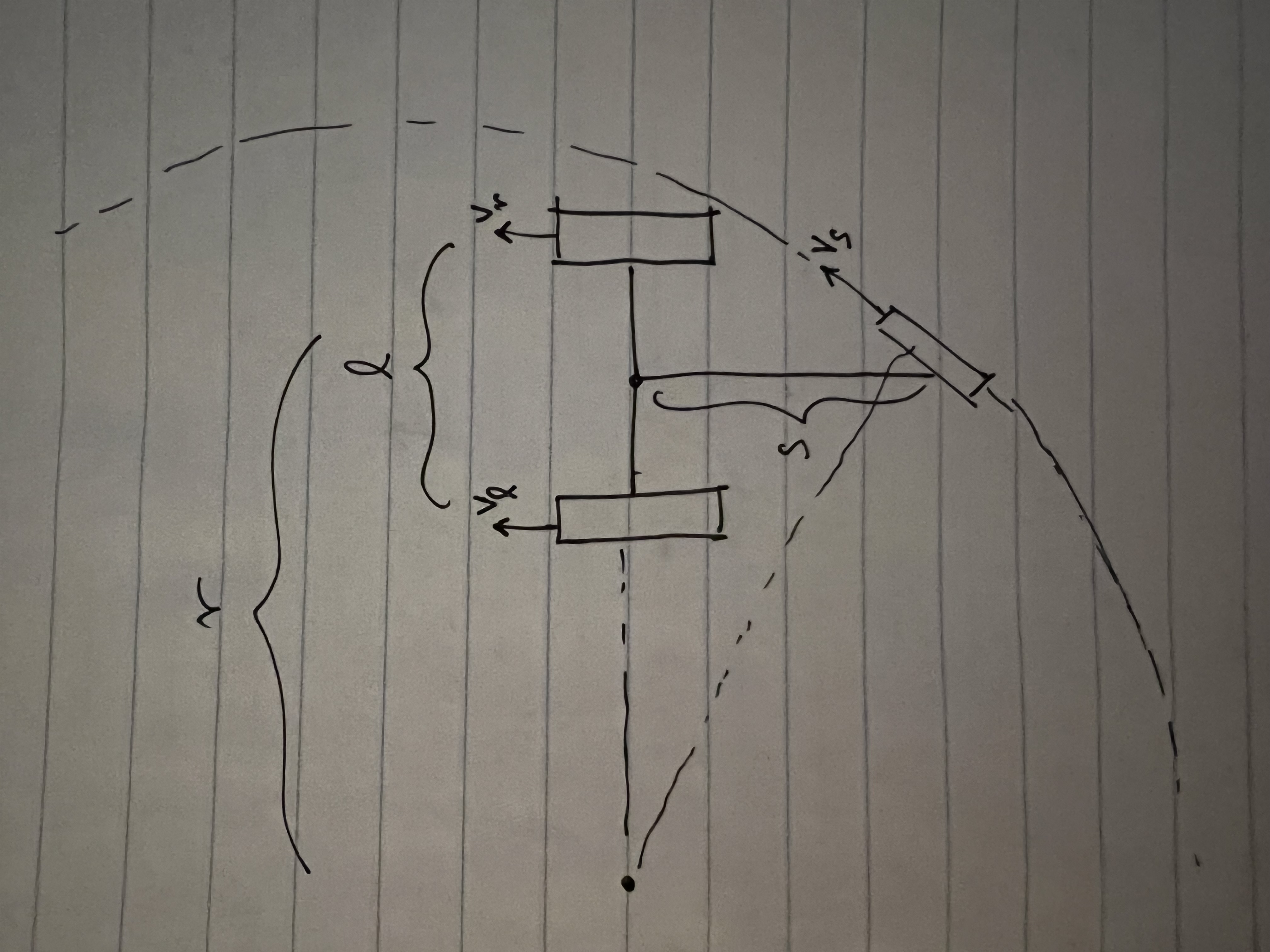
The equation can be applied to the left wheel to derive its inverse kinematics:

\[\displaylines{\vec{v_l} = \vec{v} + \vec{\omega} \times \vec{r_l} \\ = \mathbf{v + \omega (r - \frac{l}{2})}}\]

where \(r\) is the turn radius and \(l\) is the width of the robot's front axle. Applied to the right wheel, the equation yields:

\[\displaylines{\vec{v_r} = \vec{v} + \vec{\omega} \times \vec{r_r} \\ = \mathbf{v + \omega (r + \frac{l}{2})}}\]

Applied to the swerve wheel, the equation yields:

\[\displaylines{\vec{v_s} = \vec{v} + \vec{\omega} \times \vec{r_s} \\ = \mathbf{v + \omega \sqrt{r^2 + s^2}}}\]

where \(s\) is the length of the chassis (the distance between the front axle and swerve wheel).

The angle of the swerve wheel can then be calculated like so using the geometry of the robot:

\[\displaylines{\theta = \frac{\pi}{2} - tan^{-1}\left( \frac{s}{r} \right)}\]

Mathematically/intuitively, the equations check out as well. When only rotating (\(v = 0\)), \(r = \frac{v}{\omega} = \frac{0}{\omega} = 0\), so:

\[\displaylines{ v_l = v + \omega(r - \frac{l}{2}) = \omega \cdot -\frac{l}{2} \\ v_r = v + \omega(r + \frac{l}{2}) = \omega \cdot \frac{l}{2} \\ v_s = v + \omega\sqrt{r^2 + s^2} = \omega \cdot \sqrt{ s^2} = \omega \cdot s}\]

In all three cases, \(v = \omega \cdot r\), where \(r\) is the distance from each wheel to the "center of the robot", defined as the midpoint of the front axle. Since rotating without translating will be around a center of rotation equal to the center of the robot, the previous definition for \(r\) can be used.

As for the equation for \(\theta\), the angle of the swerve wheel, it checks out intuitively as well. When only translating (driving straight: \(\omega = 0\)), \(r = \frac{v}{\omega} = \frac{v}{0} = \infty\), so:

\[\displaylines{ \theta = \frac{\pi}{2} - tan^{-1} \left( \frac{s}{r} \right) \\ = \frac{\pi}{2} - tan^{-1} \left( \frac{s}{\infty} \right) \\ = \frac{\pi}{2} - tan^{-1}(0) \\ = \frac{\pi}{2} - 0 \\ = \frac{\pi}{2} }\]

As expected, when translating, \(\theta = 0\), as the swerve wheel must point straight for the robot to drive straight. When only rotating (\(v = 0\)), \(r = \frac{v}{\omega} = \frac{0}{\omega} = 0\), so:

\[\displaylines{ \theta = \frac{\pi}{2} - tan^{-1} \left( \frac{s}{r} \right) \\ = \frac{\pi}{2} - tan^{-1} \left( \frac{s}{0} \right) \\ = \frac{\pi}{2} - tan^{-1}(\infty) \\ = \frac{\pi}{2} - \lim_{x \to +\infty} tan^{-1}(x) \\ = \frac{\pi}{2} - \frac{\pi}{2} \\ = 0}\]

As expected, when only translating (driving straight), \(\theta = \frac{\pi}{2}\), or in other words, the swerve wheel is pointed directly forwards to drive the robot directly forwards. When only rotating, \(\theta = 0\), or in other words, the swerve wheel is pointed directly to the right to allow the robot to rotate counterclockwise.

Next Steps:

The next step is to use PID control to maintain target velocities and angles calculated using the derived inverse kinematic equations. Then, these equations can be used in future motion planning/path planning attempts to get the robot to follow a particular desired \(v\) and \( \omega\).

A distance sensor will also need to be used to calculate \(s\), the distance between the front axle and swerve wheel of the robot.