21 Jan 2023
League Meet #3 Review
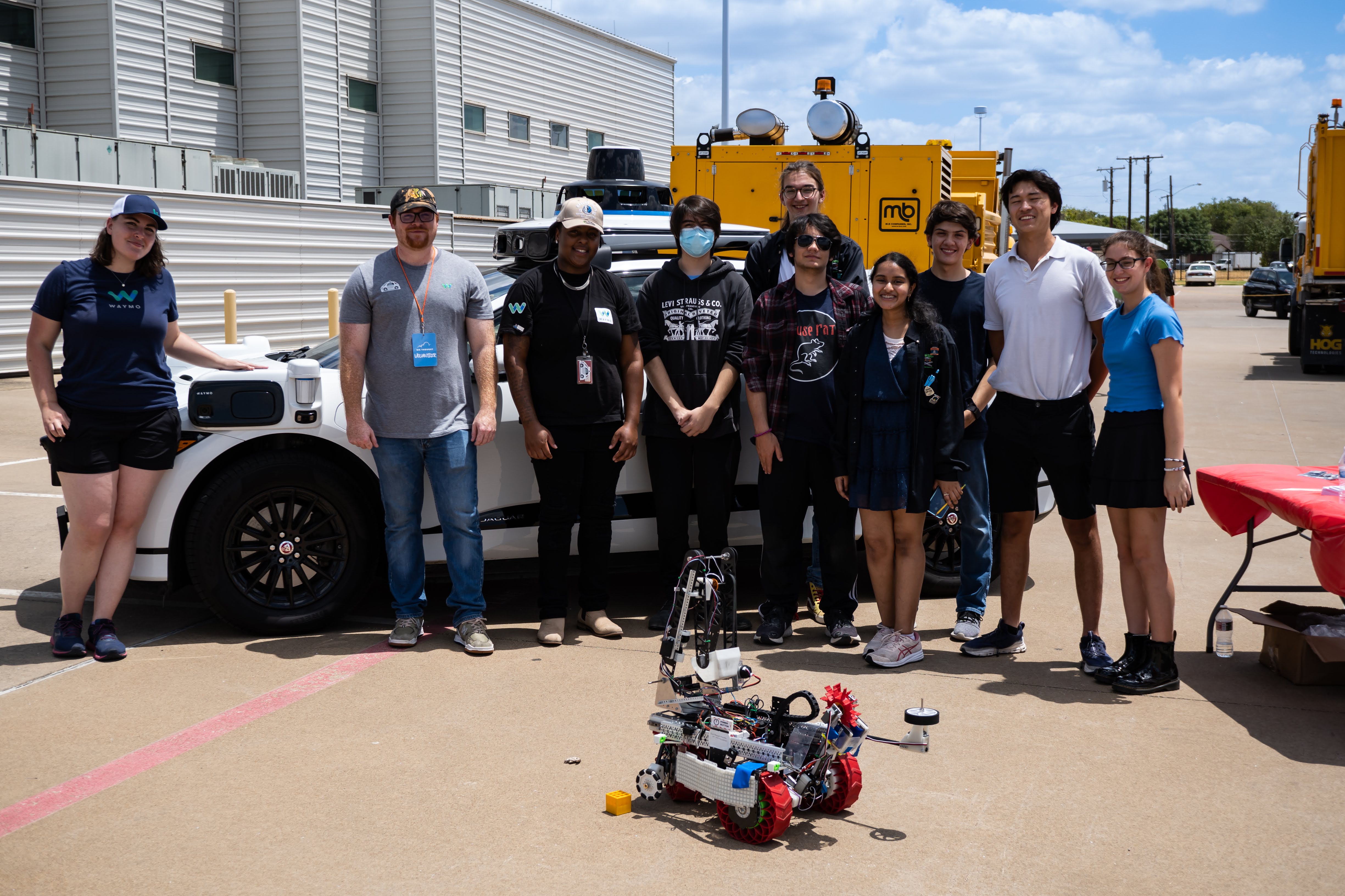
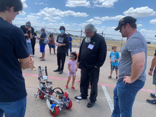
By Aarav, Anuhya, Gabriel, Leo, Vance, Trey, and Georgia
Task: Review our performance at the 3rd League Meet and discuss possible next steps
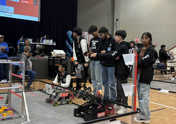
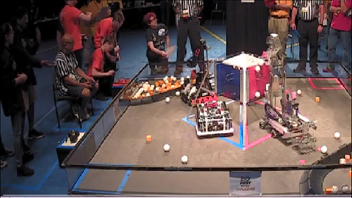
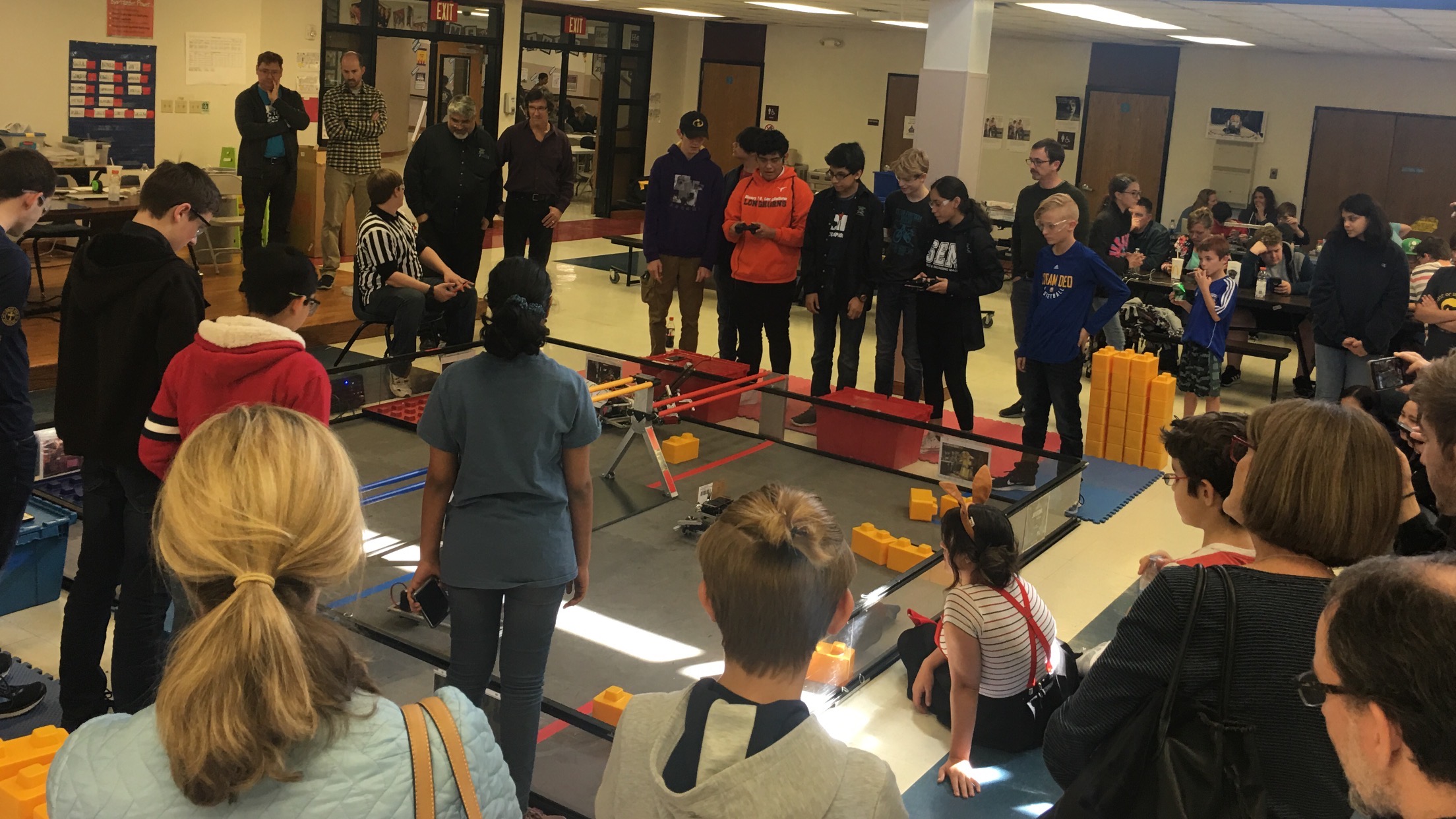
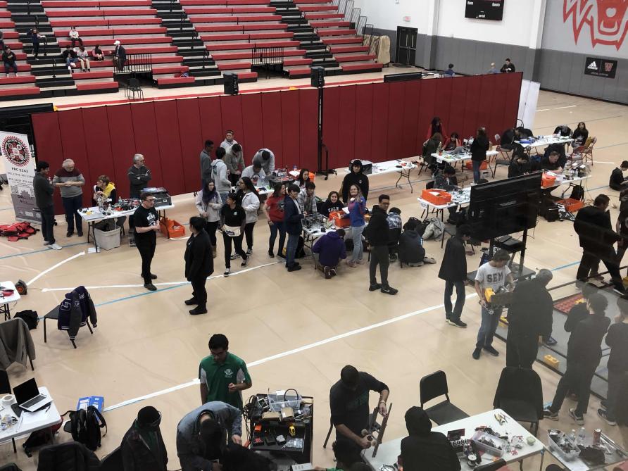
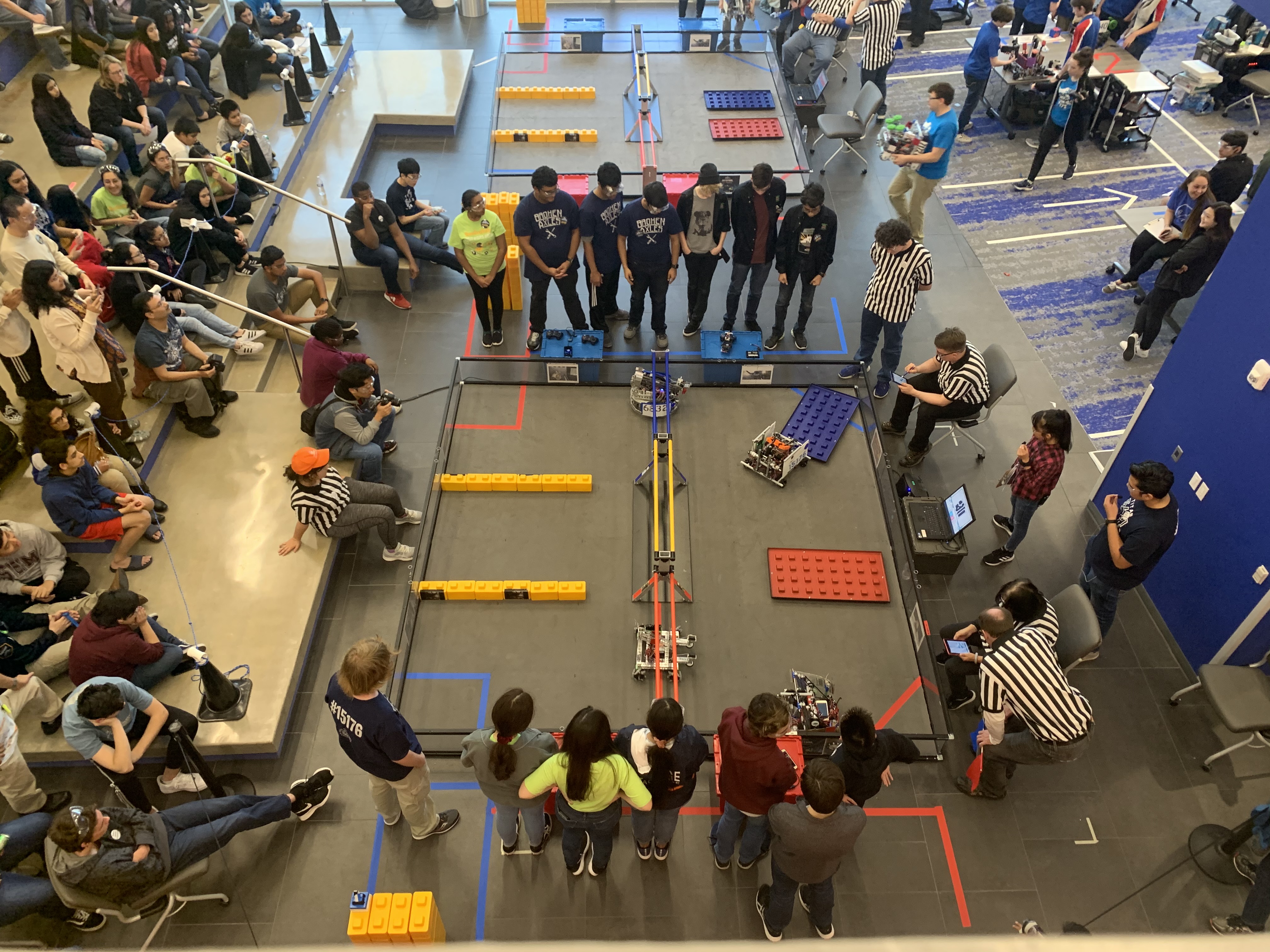
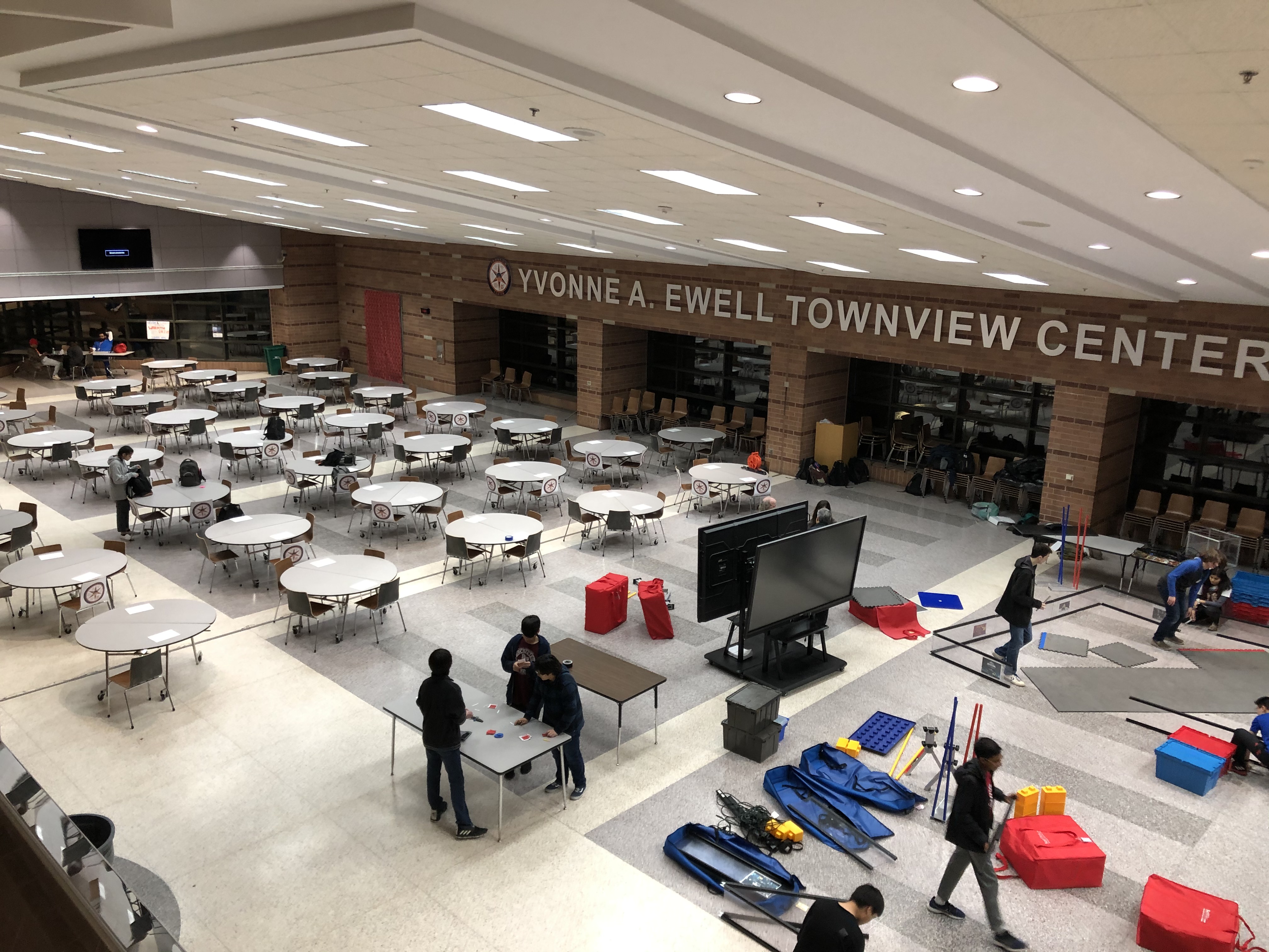
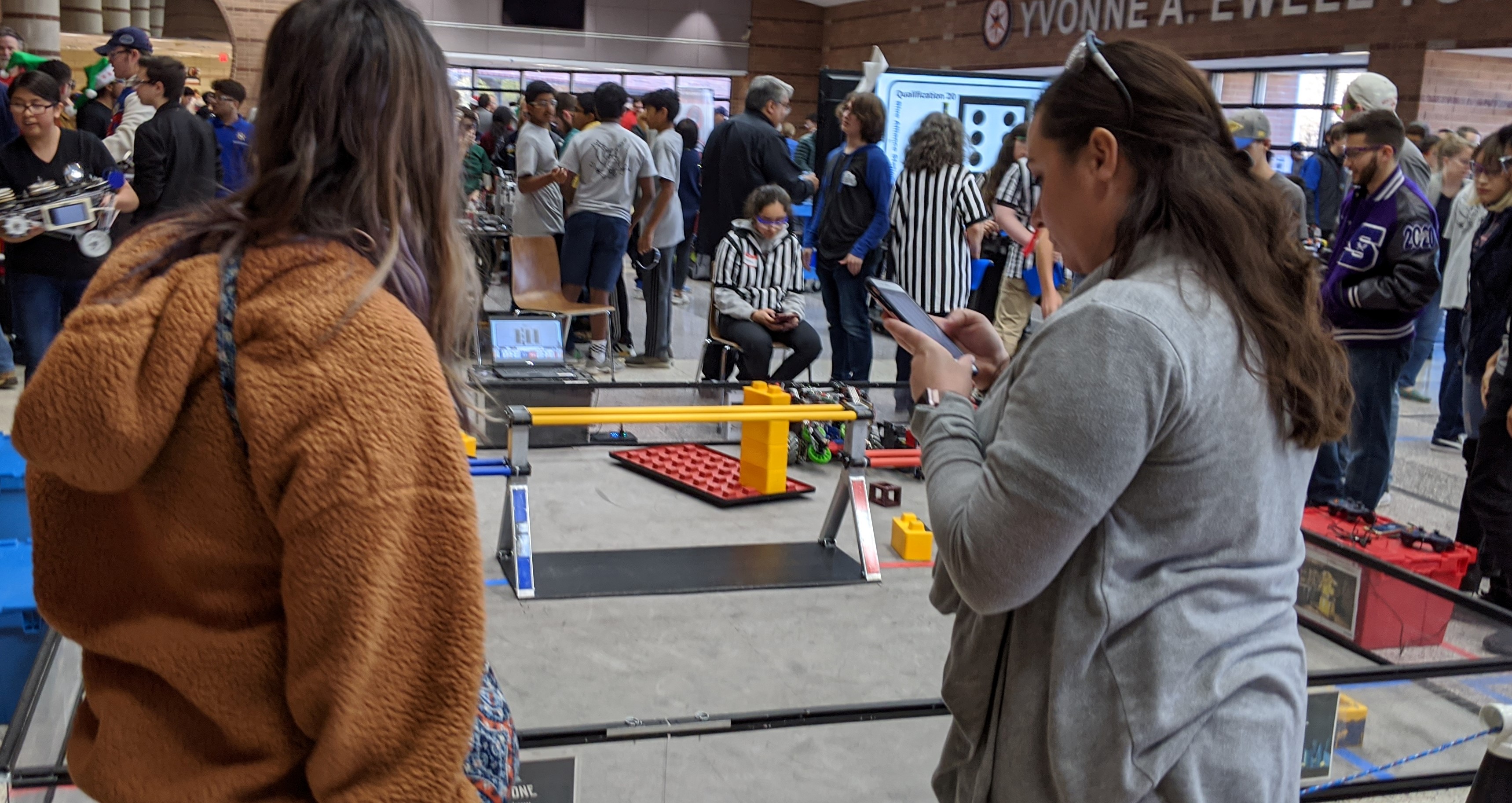
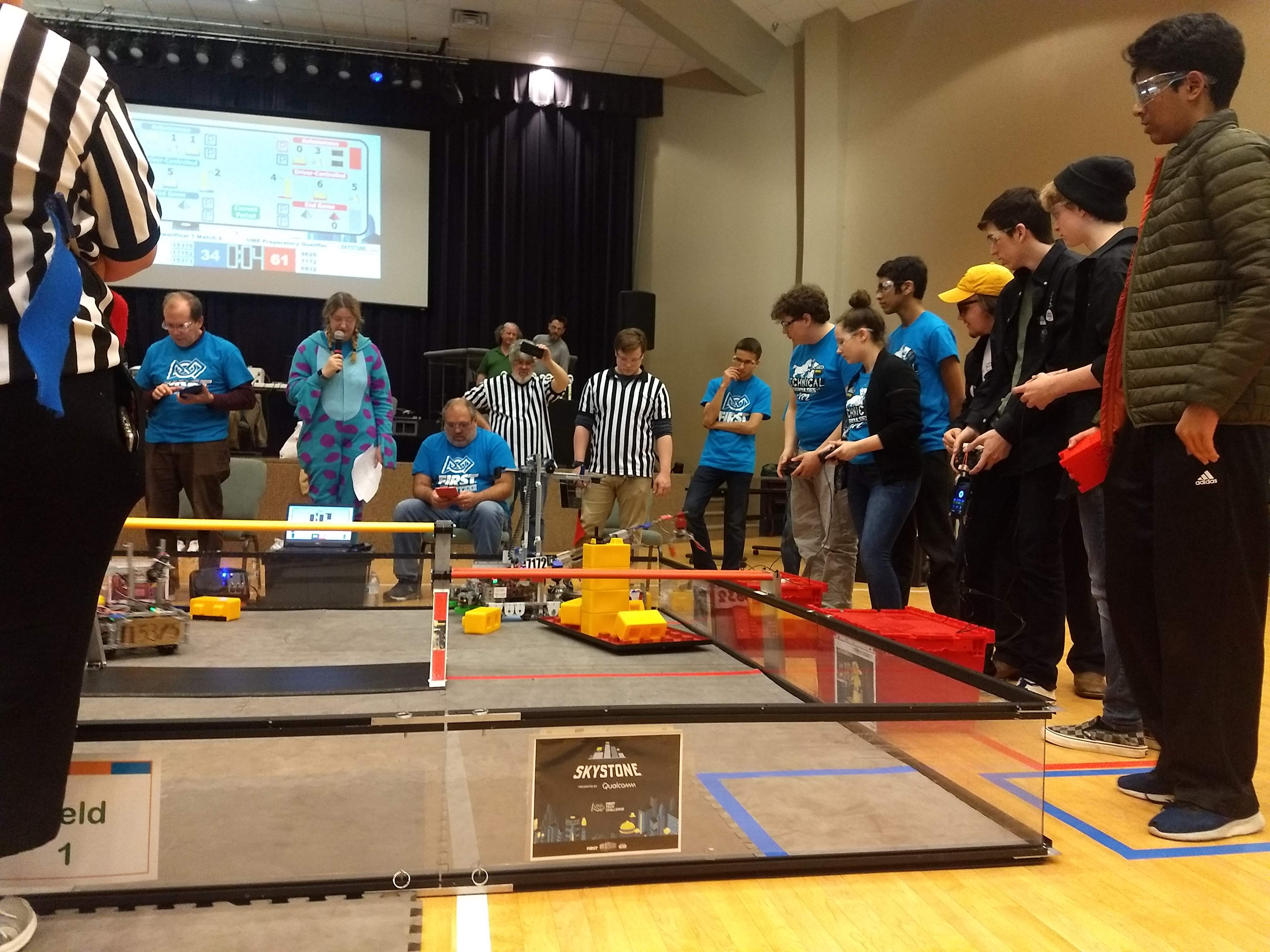
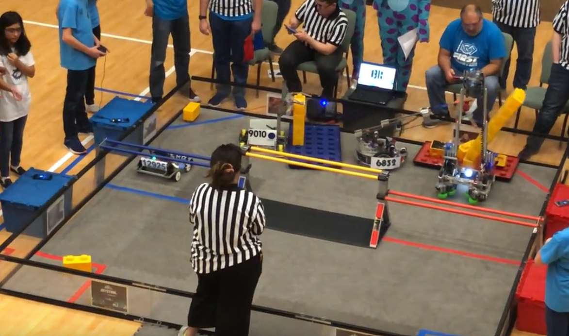
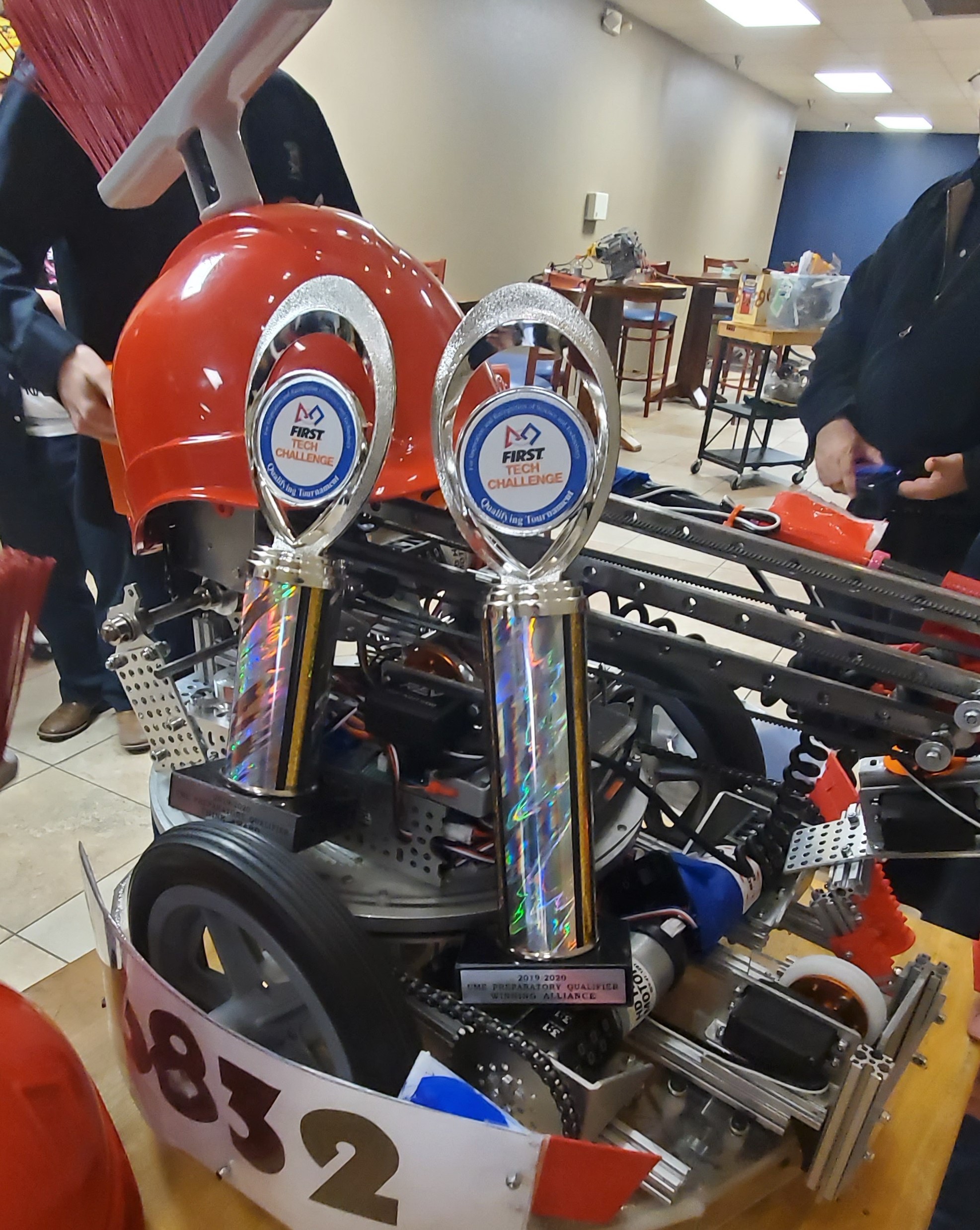
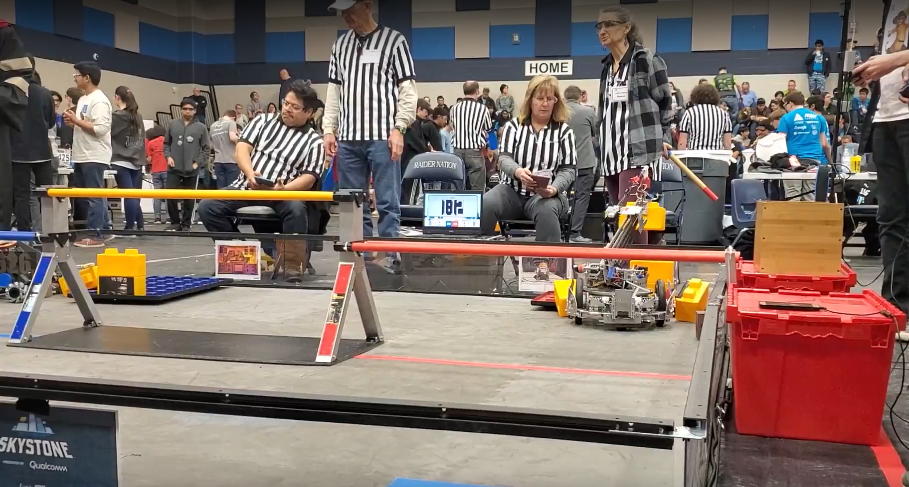
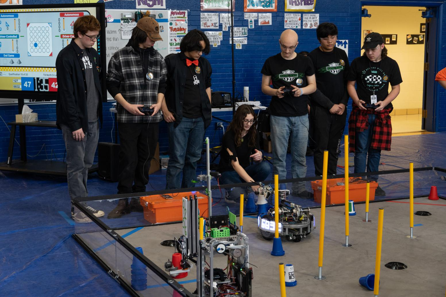
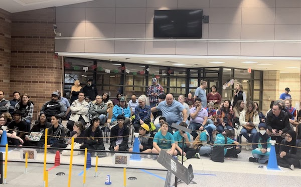
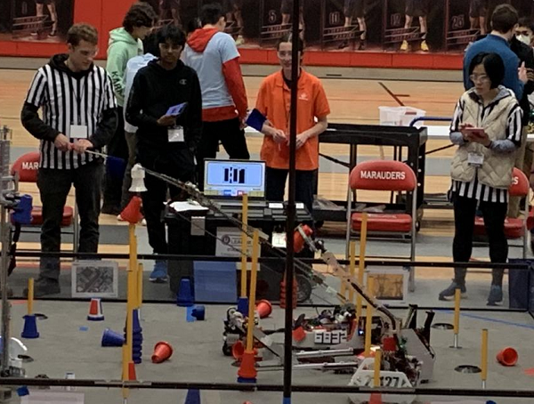
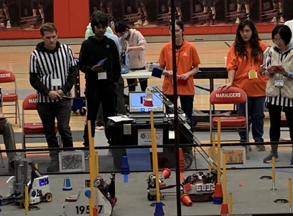
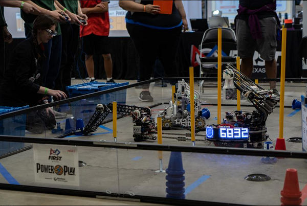
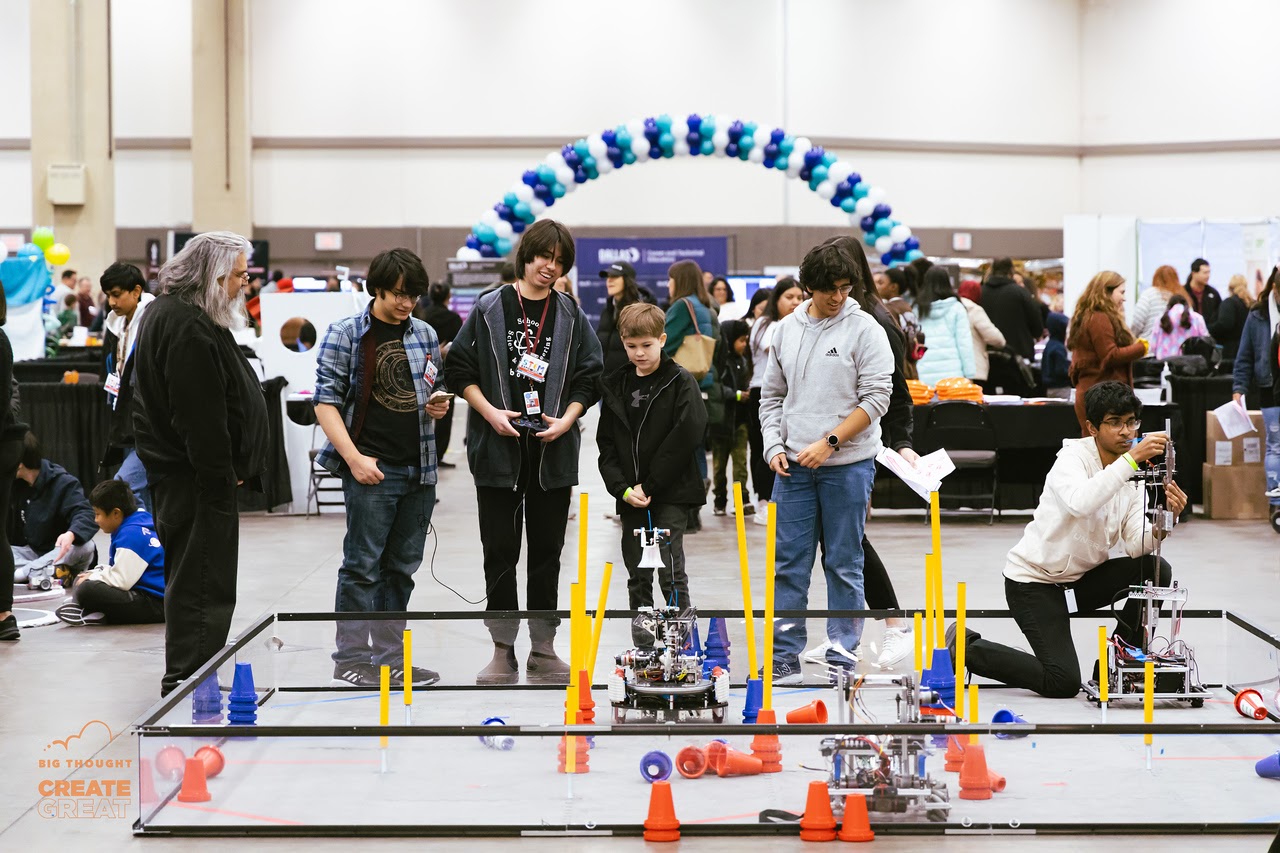
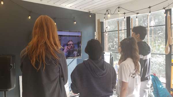
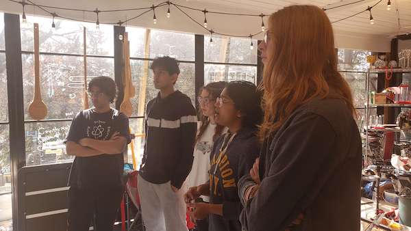
Today, Iron Reign and our two sister teams participated in the 3rd League Meet for the U League at UME Preparatory for qualification going into the Tournament next week. Overall, we did solid, going 4-2 at the meet; however, we lost significant tiebreaker points in autonomous points due to overall unreliability. At the end of the day, we didn’t do as great as we would have liked, but we did end the meet ranked #2 in the U League in #5 between both the D and U Leagues, and got some valuable driver practice and code development along the way.
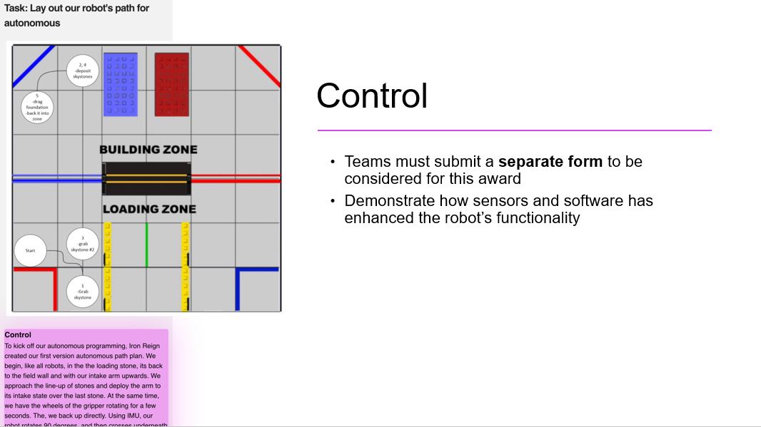
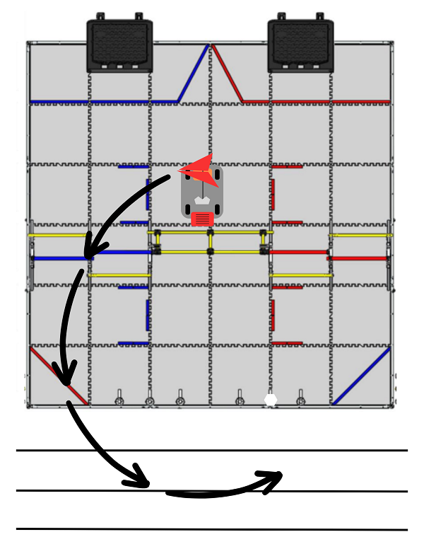
We entered the meet with brand new autonomous code that allowed us to ideally score three cones in autonomous and park, equating to about 35 points.
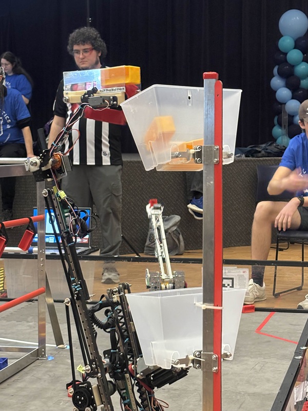
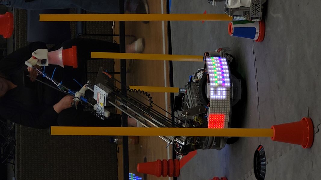
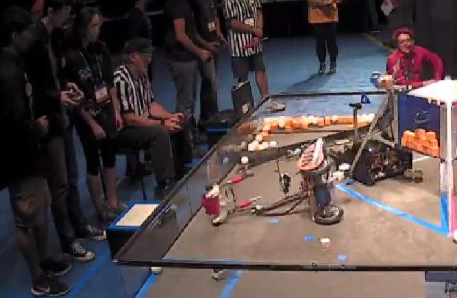
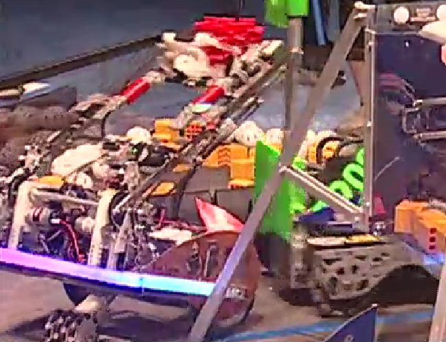
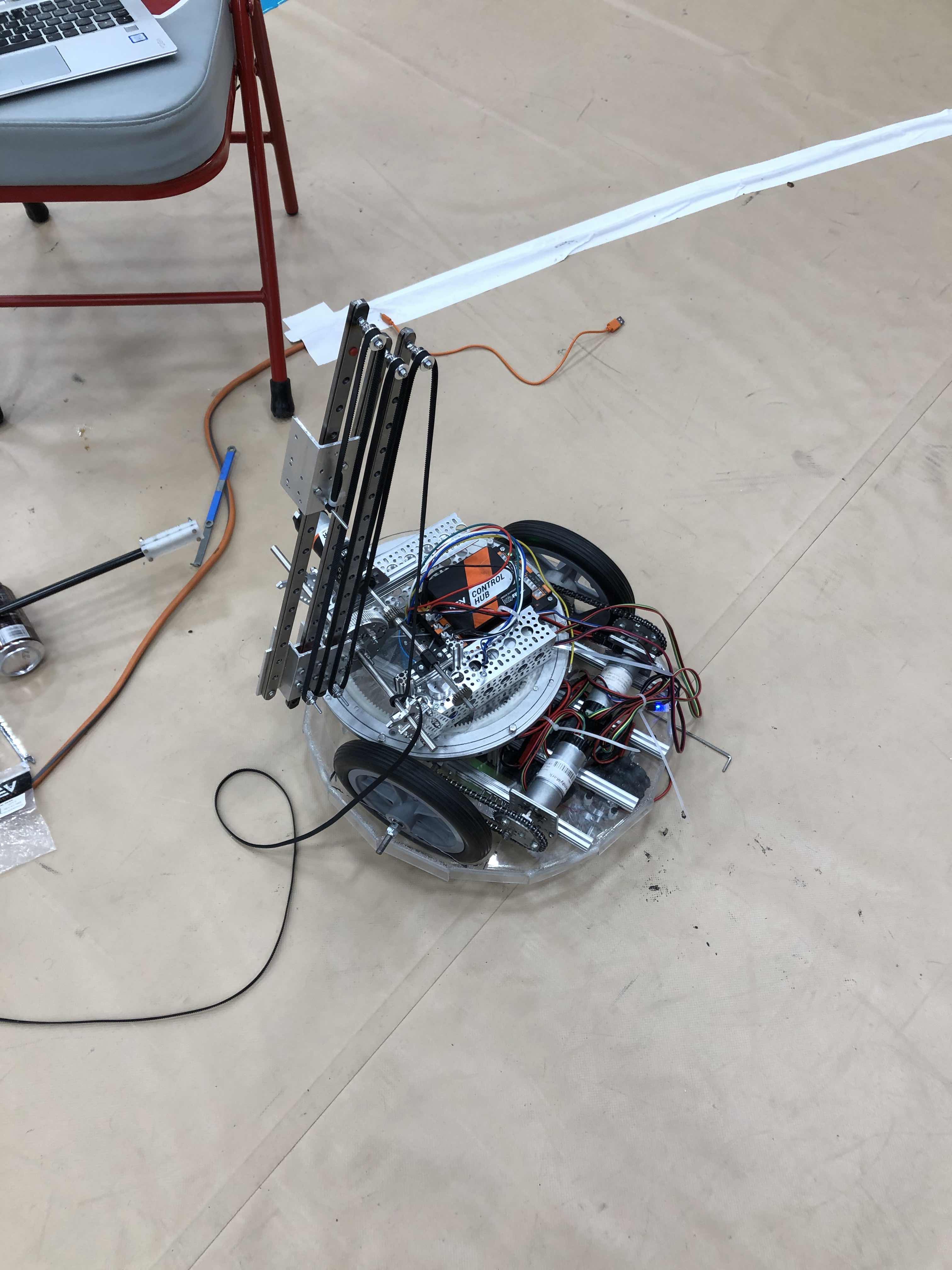
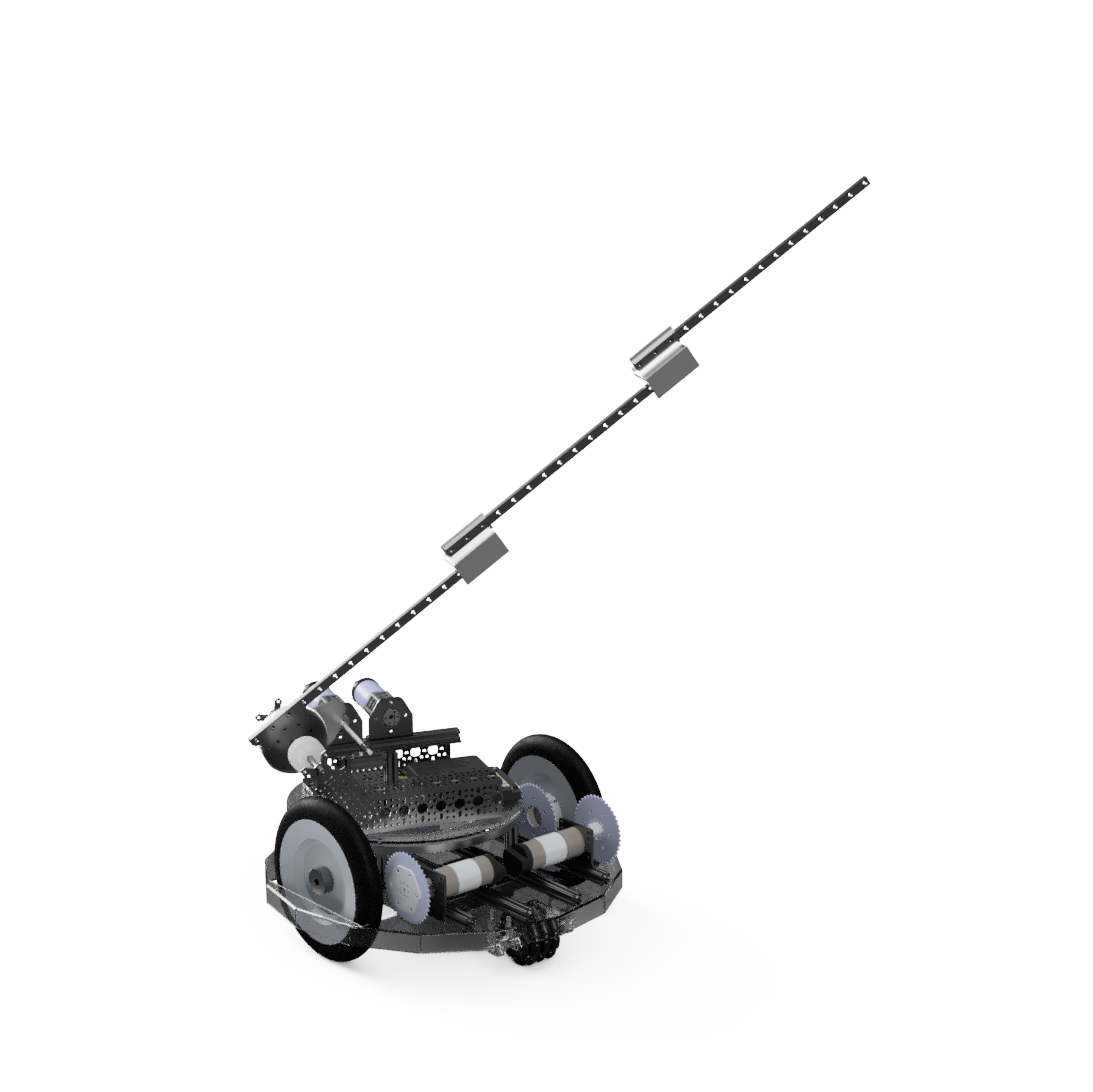
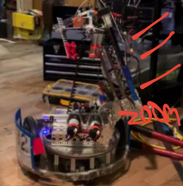
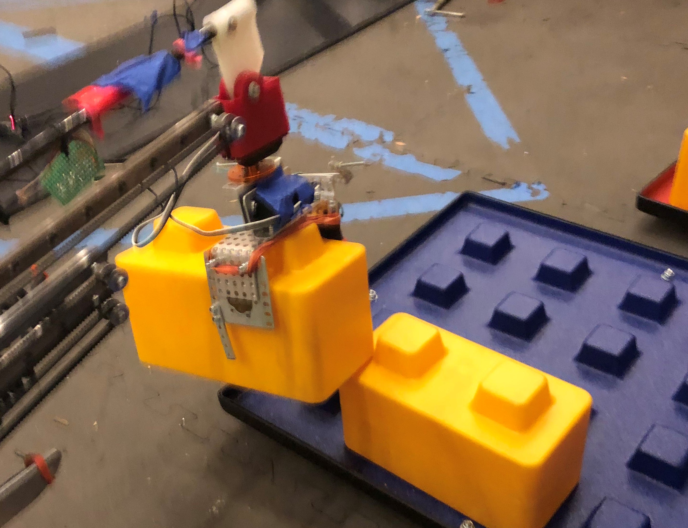
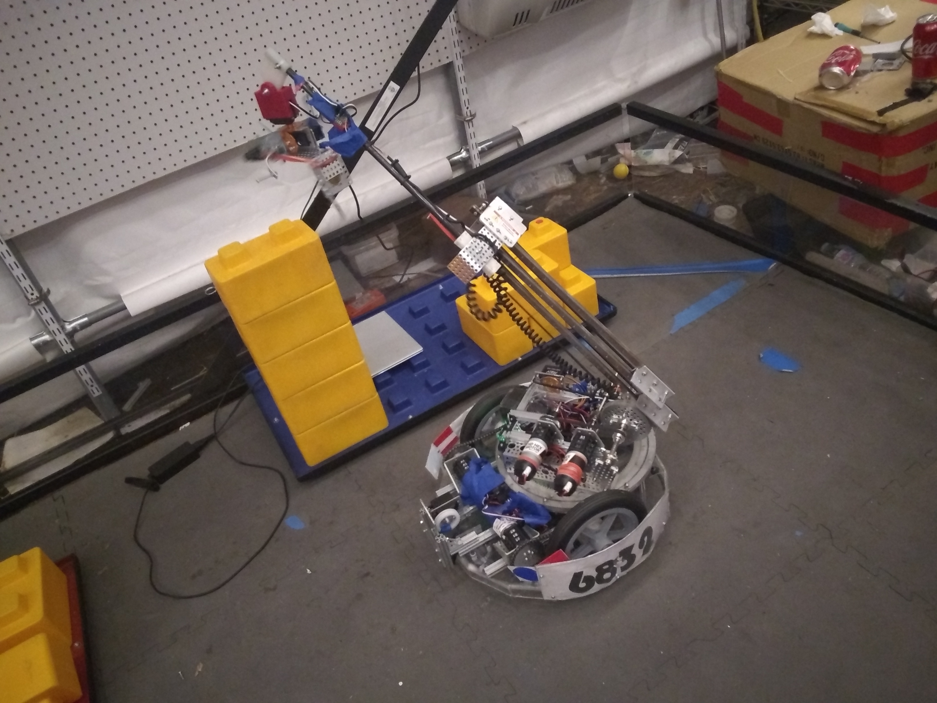
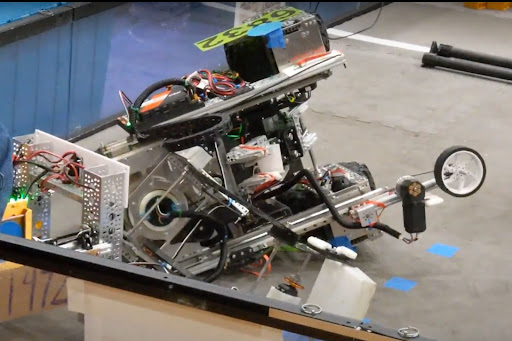
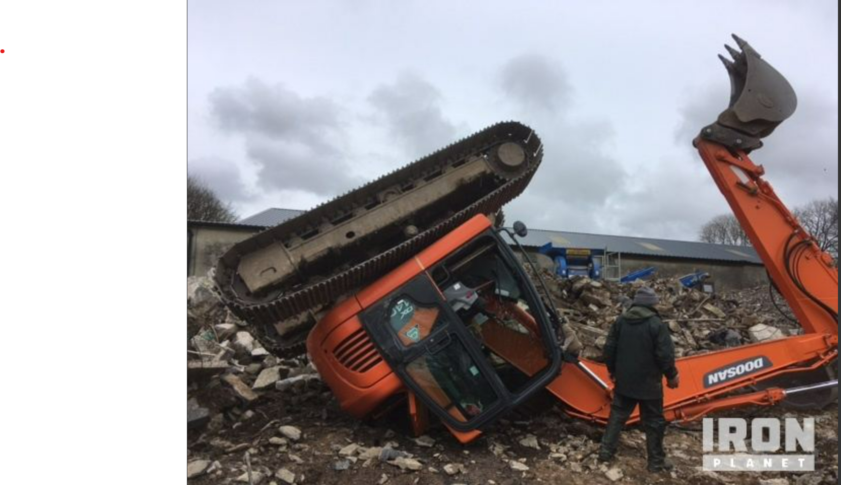
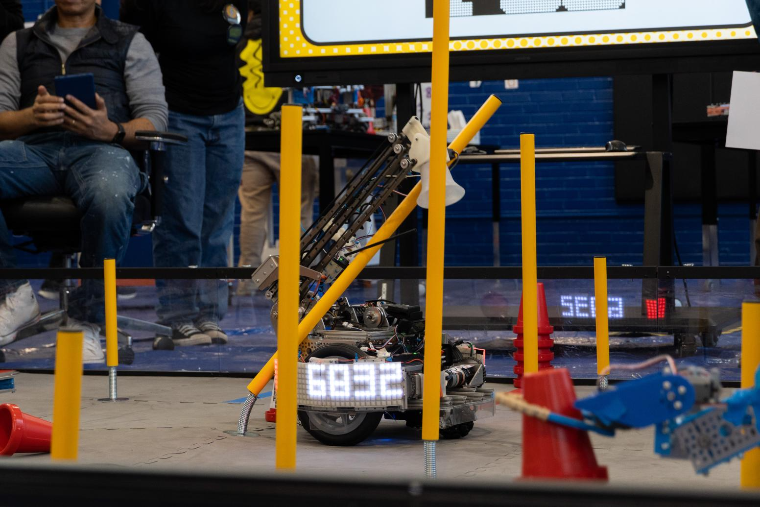
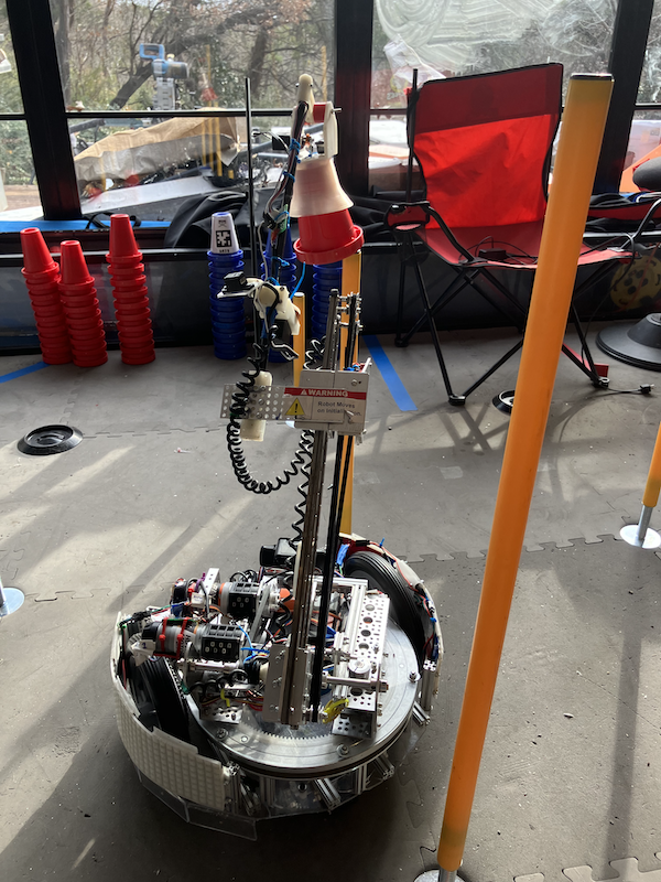
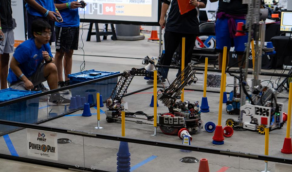
Another main issue that plagued us was tipping, as our robot tipped over in practice and in an actual match due to the extension of the arm and constant erratic movement, which we will elaborate on in the play-by-play section.
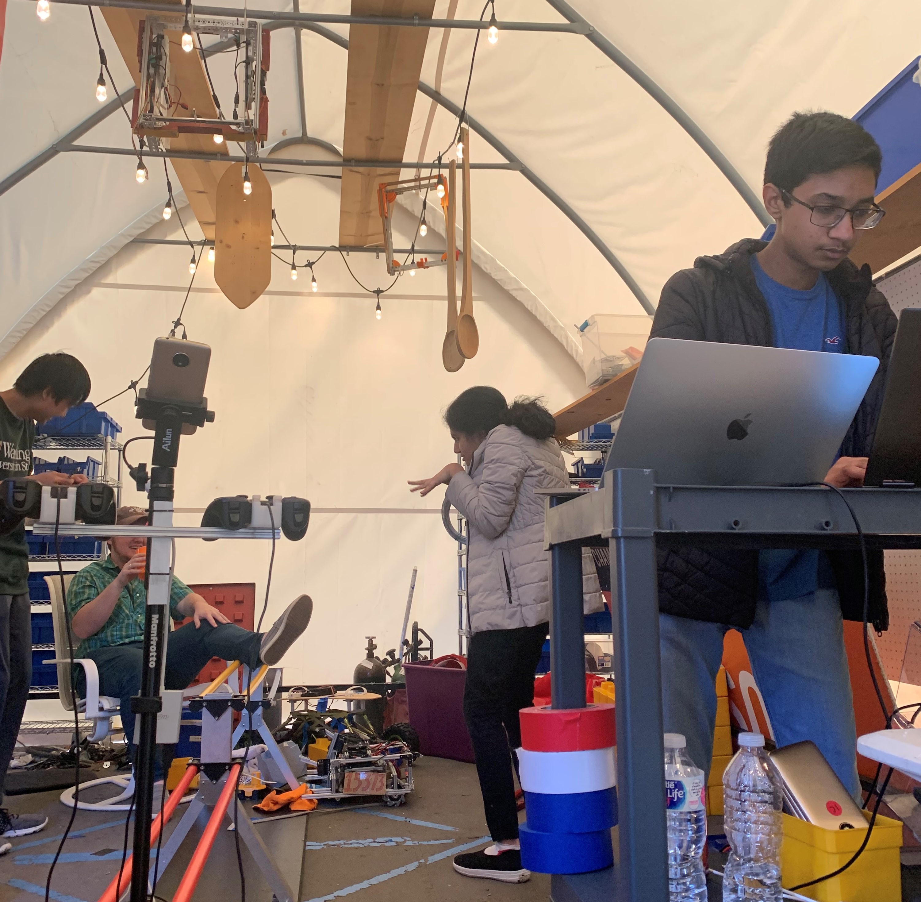
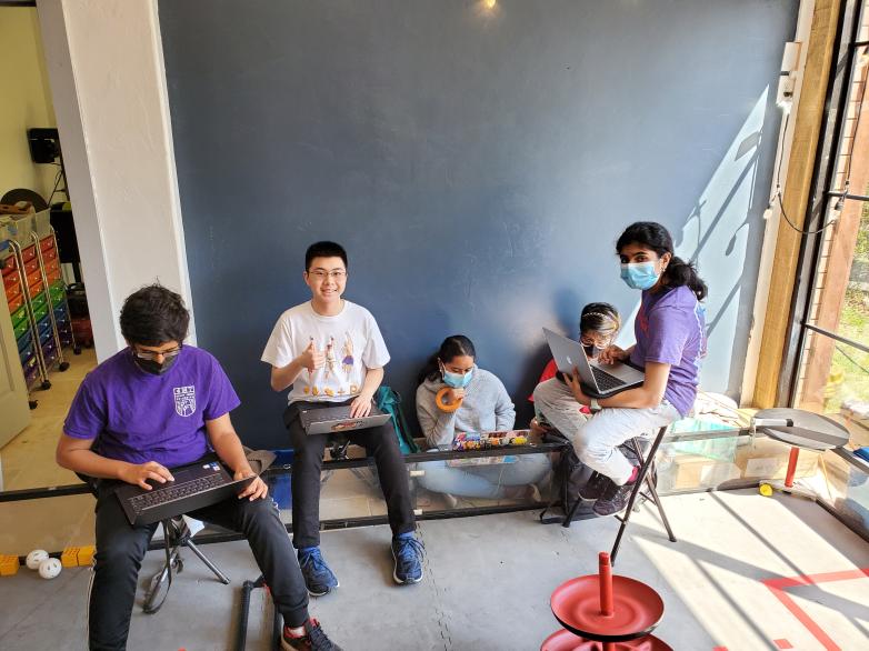
We also want to preface that much of our code and drive teams were running on meager amounts of sleep due to late nights working on TauBot2, so a lot of the autonomous code and river error can be attributed to fatigue caused by sleep deprivation. Part of our takeaways from this meet is to avoid late nights as much as possible, stick to a timeline, and get the work done beforehand.
Play by Play
Match 1: 46 to 9 Win
In the autonomous section, our robot missed the initial preload cone and fell short of grabbing cones from the cone stack because there was an extra cone. Finally, our robot overshot the zone and got no parking points. Overall, we scored 0 points.
In the tele-op and endgame sections, because of a poor quality battery that was overcharged at around 13.9 volts, our entire shoulder and arm stopped functioning and just stood stationary for the whole period. In the end, we only scored 2 points by parking in the corner. However, due to the extra cone on the cone stack at the beginning of autonomous, we were granted a rematch.
In the autonomous of the rematch, our preload cone dropped to the side of the tall pole, but we could grab and score one cone on the tall pole, missing the second one. However, it did not fully move into Zone 3, meaning we didn’t get any parking points. Overall, 5 points in auton.
In the tele-op and endgame, we scored two cones on the tall poles and one on a medium pole, which equates to 20 points in that section, including six ownership points.
Total Points: 29
Analysis: We need to ensure that our battery does not have too high of a voltage because that causes severe performance impacts. More autonomous tuning is also required to score both cones and properly park. Our light battery also died in the middle of the second match due to low charge, which will need to be taken care of in the future since that can lead to major penalties.
Match 2: 68 to 63 Loss
In the autonomous section, our robot performed great and went according to plan, scoring the preload cone and 2 more on the tallest cone and parking, equating to 35 points.
However, in the tele-op and endgame, the robot’s issues reared their ugly heads. We did score one cone on a tall cone and one on a medium cone. However, after our opponent took ownership of one of our tall poles, we went for another pole instead of taking it back, and that led to us tipping over as the arm extended, which ended the game for us. We did not incur any penalties but had we scored that cone and taken back our pole, we would have won and gotten to add a perfect autonomous to our tiebreaker points. We ended up scoring 9 points in this section.
Total Points: 44
Analysis: Excellent autonomous performance marred by a tipping issue and sub-par driver performance. The anti-tipping code did not work as intended, and that issue will need to be fixed to allow TauBot to score at its entire range.
Match 3: 78 to 31 Win
In the autonomous section, we missed the preload cone and couldn’t grab both the cones on the stack, and we also did not park as our arm and shoulder crossed the border. As a result, we scored 0 points total in this section.
In the tele-op and endgame section, we scored a lot better, scoring two cones on the tall poles, one on the medium poles, and two on the short ones. This, including our 15 ownership points, equates to a total of 35 points.
Total Points: 35
Analysis: The autonomous does need tuning to at least park because of the value of autonomous points. Our lack of driver practice is also slightly evident in the time it takes to pick up new cones, but that can be solved through increased gameplay.
Match 4: 40 to 32 Win
In the autonomous section, we scored our preload cone on a tall pole, but intense arm oscillation meant we missed the first cone from the stack on drop-off and the second cone from the stack on pickup. We also overshot parking again, bringing our total in this period to 5 points.
In the tele-op and endgame section, we scored two cones on the tall poles. So with ownership points, our total in this section was 16 points. We did miss one cone drop-off, though, and our pickups in the substation could have been better as we tipped over a couple of cones during pickup.
Total Points: 21
Analysis: Parking still needed to be tuned, but the cone scoring was a lot more consistent, but still requires a bit more work to achieve consistency. Other than that, improved driver practice will help cycle times and scoring.
Match 5: 51 to 24 Win
In the autonomous section, our arm never engaged to go and score our preload, and the robot did park, meaning we scored 20 points in this section.
In the tele-op and endgame section, we scored two cones on the tall poles, one cone on the medium poles, and missed three on drop-off. We also scored our beacon, bringing our total point count in this game portion to 30 points.
Total Points: 50
Analysis: Pretty solid match, but the autonomous still needs tuning, and driver practice on cone drop-offs could be better.
Match 6: 74 to 50 Loss
In the autonomous section, our robot missed the drop off of 2 cones but parked, bringing the total to 20 points for autonomous.
In the tele-op and endgame section, miscommunication with our alliance partner led to them knocking our cones out of the substation and blocking our intake path multiple times. We scored three cones on the tall poles and missed two on drop-off. In the end, we scored the beacon, scoring 30 points in this section.
Total Points: 50(we carried)
Analysis: Communication with our alliance partner was a significant issue in this match. Our alliance partner crossed onto our side and occupied the substation for a while, blocking our human player from placing down cones and blocking our intake path. This led to valuable seconds being wasted.
Overall, our main issues revolved around autonomous code tuning; although our autonomous performance did improve, poor driver practice we chalk up to fatigue, along with minor tipping and communication issues. However, we plan to understand what happened and solve our problems before the next week’s Tournament.
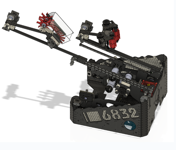
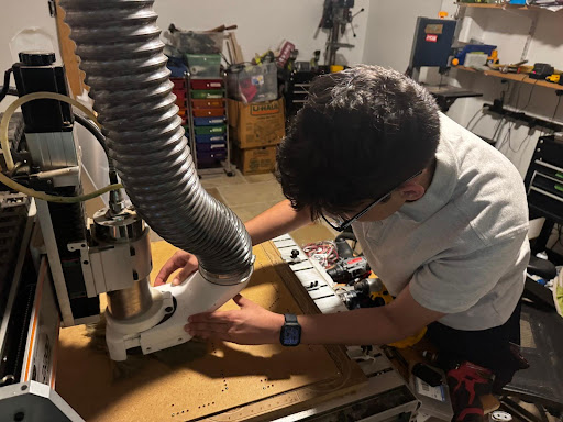
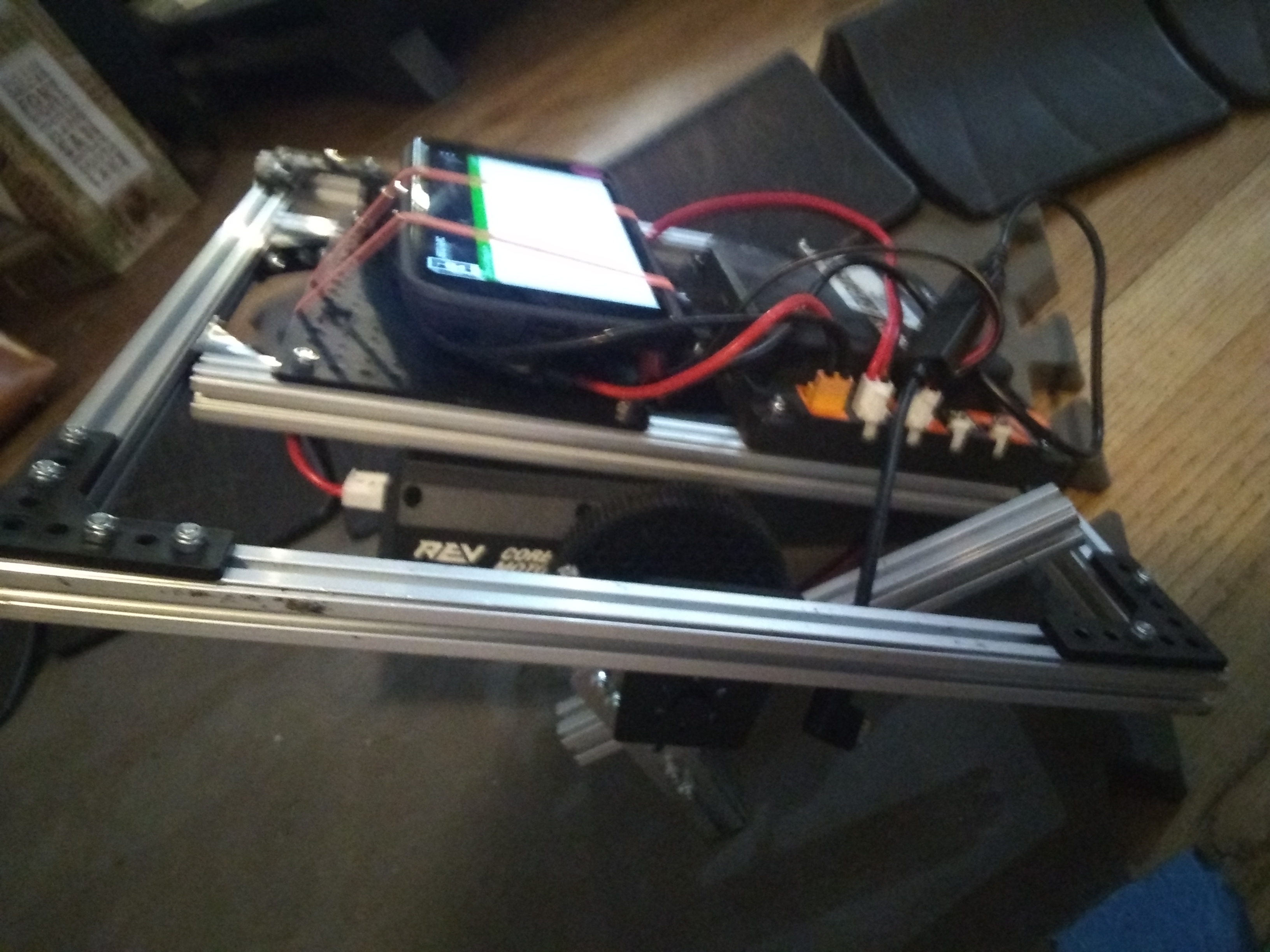
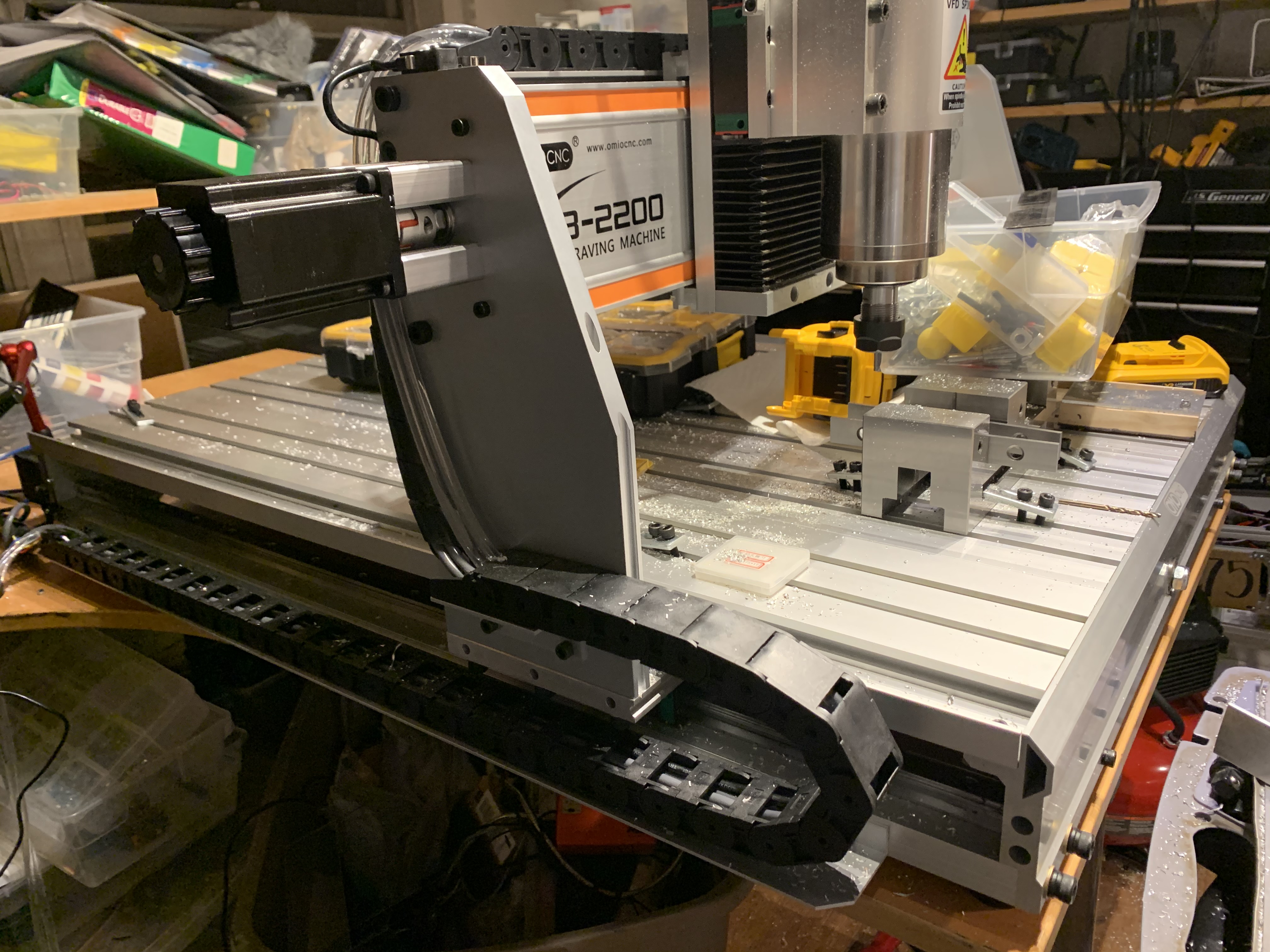
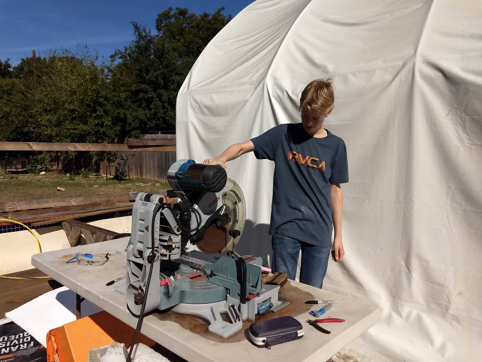
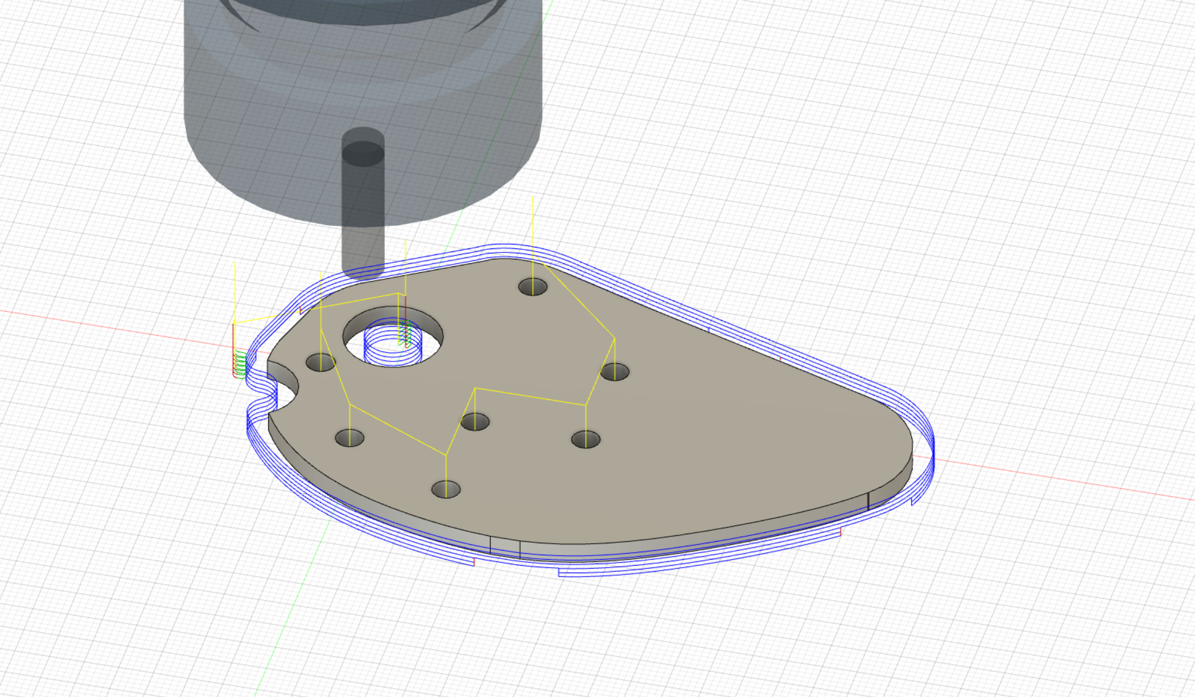
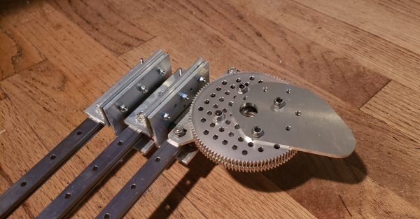
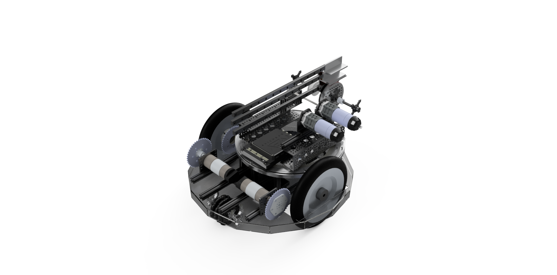
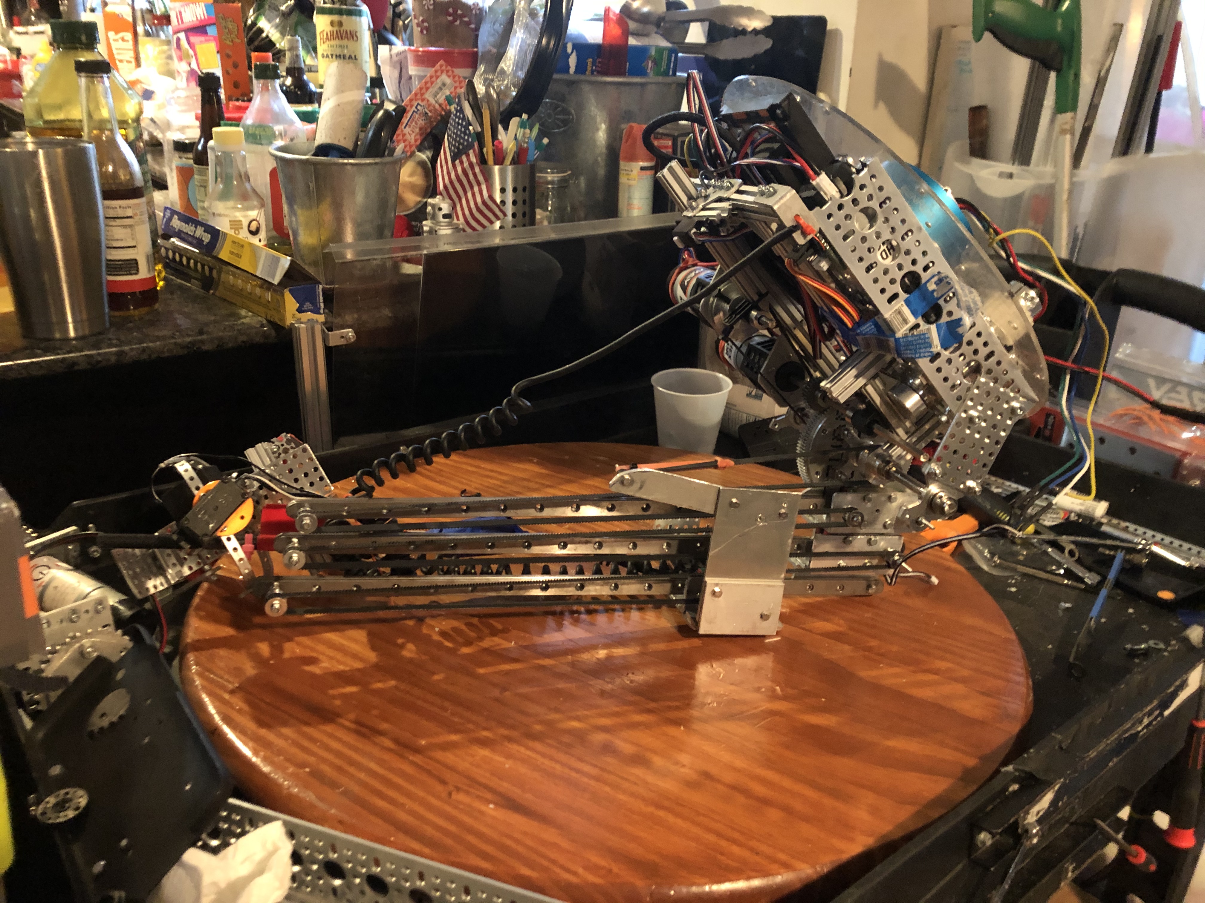
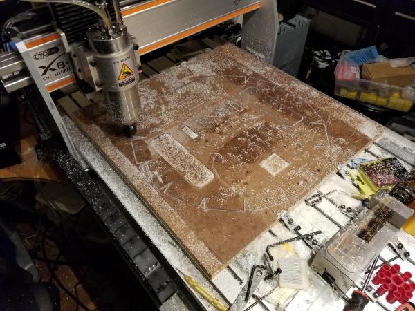
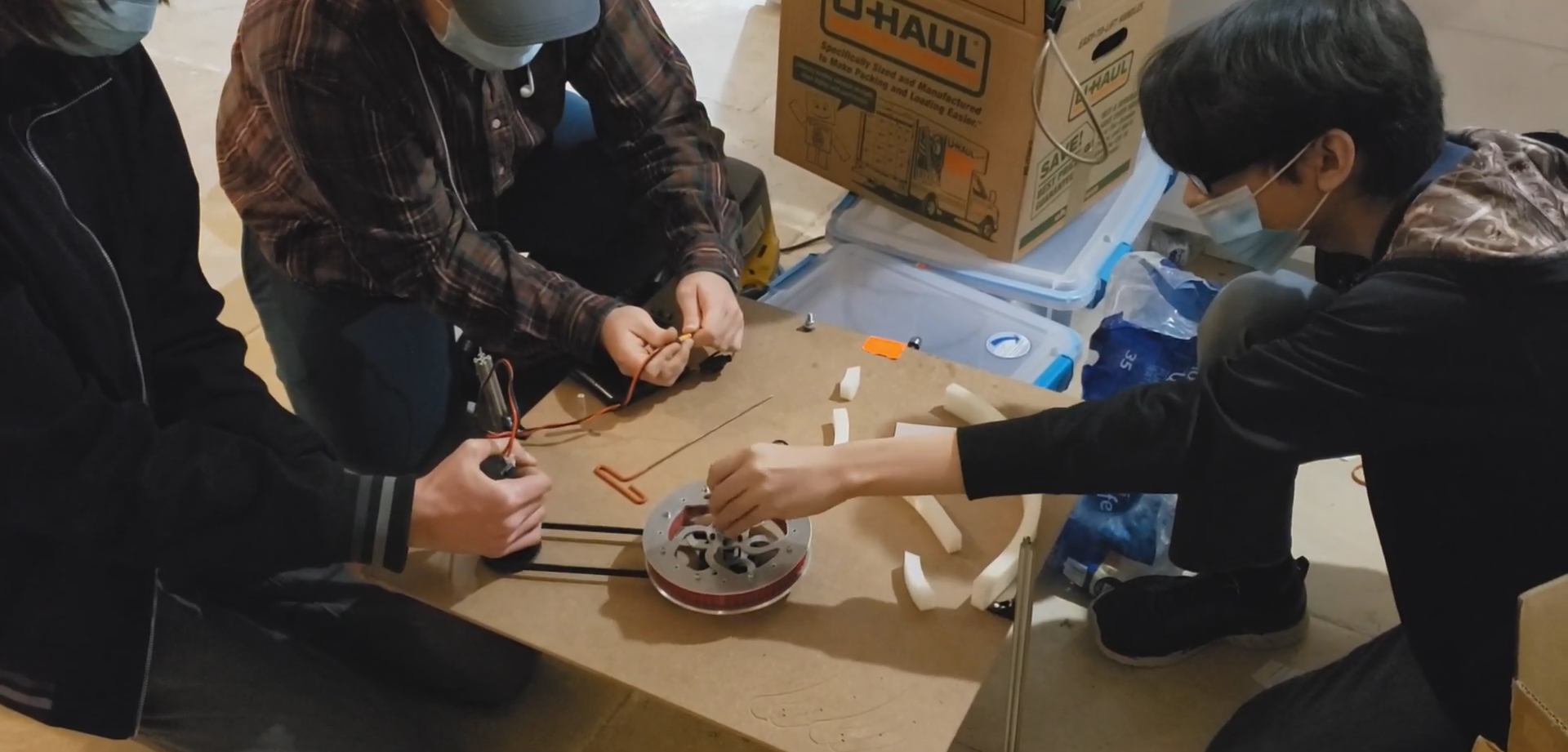
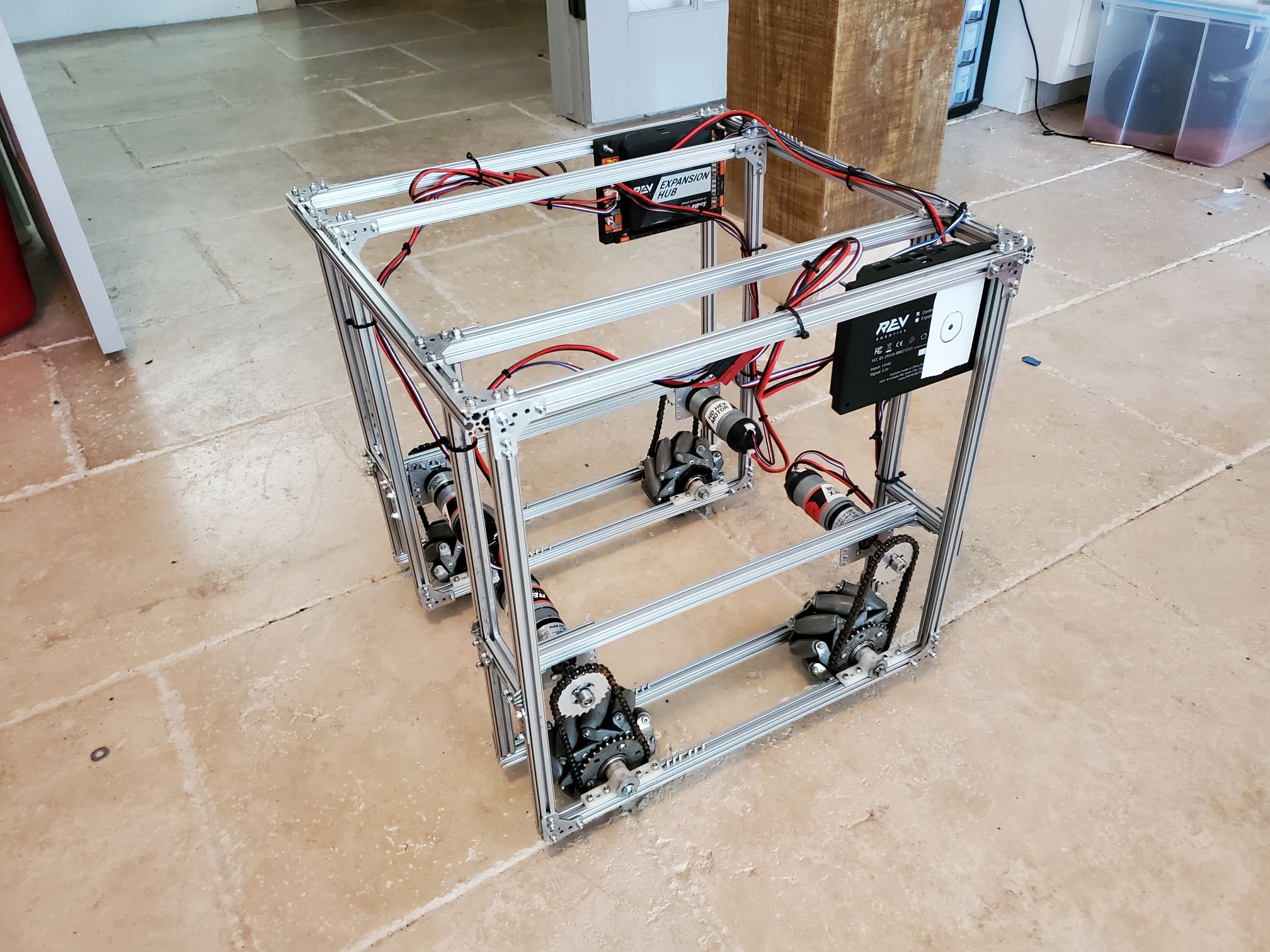
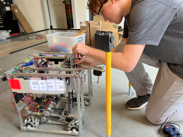
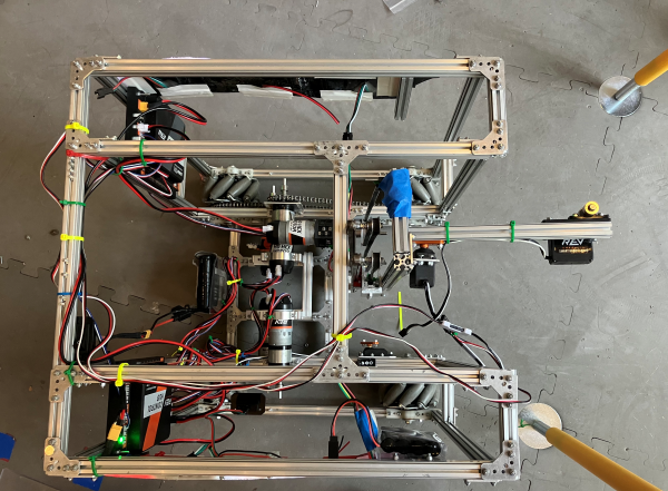
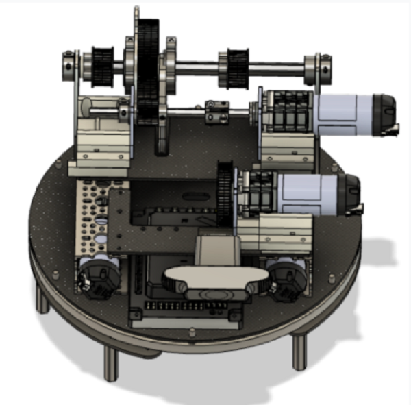
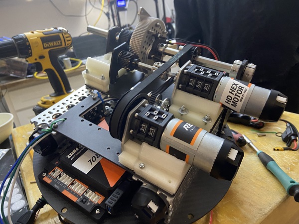
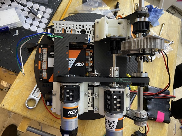
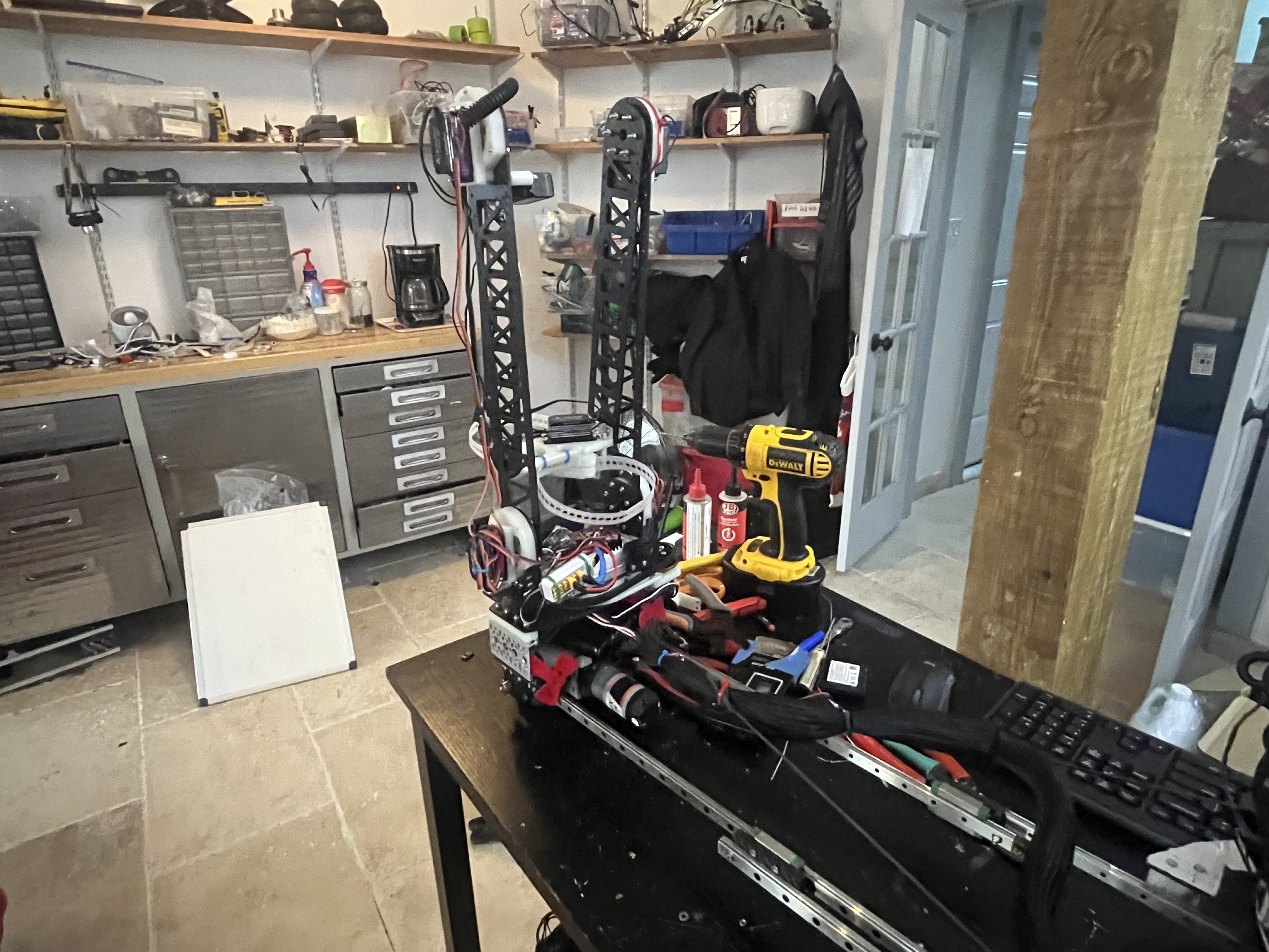
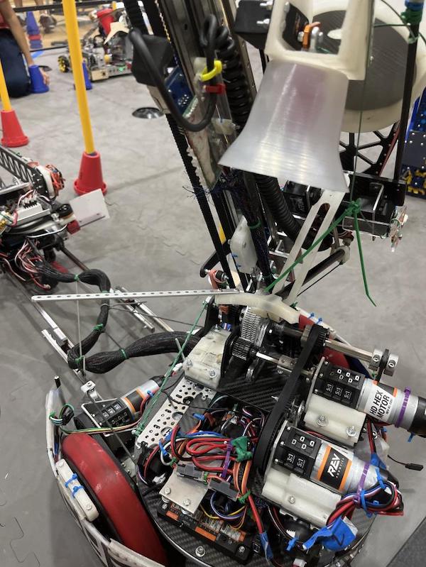
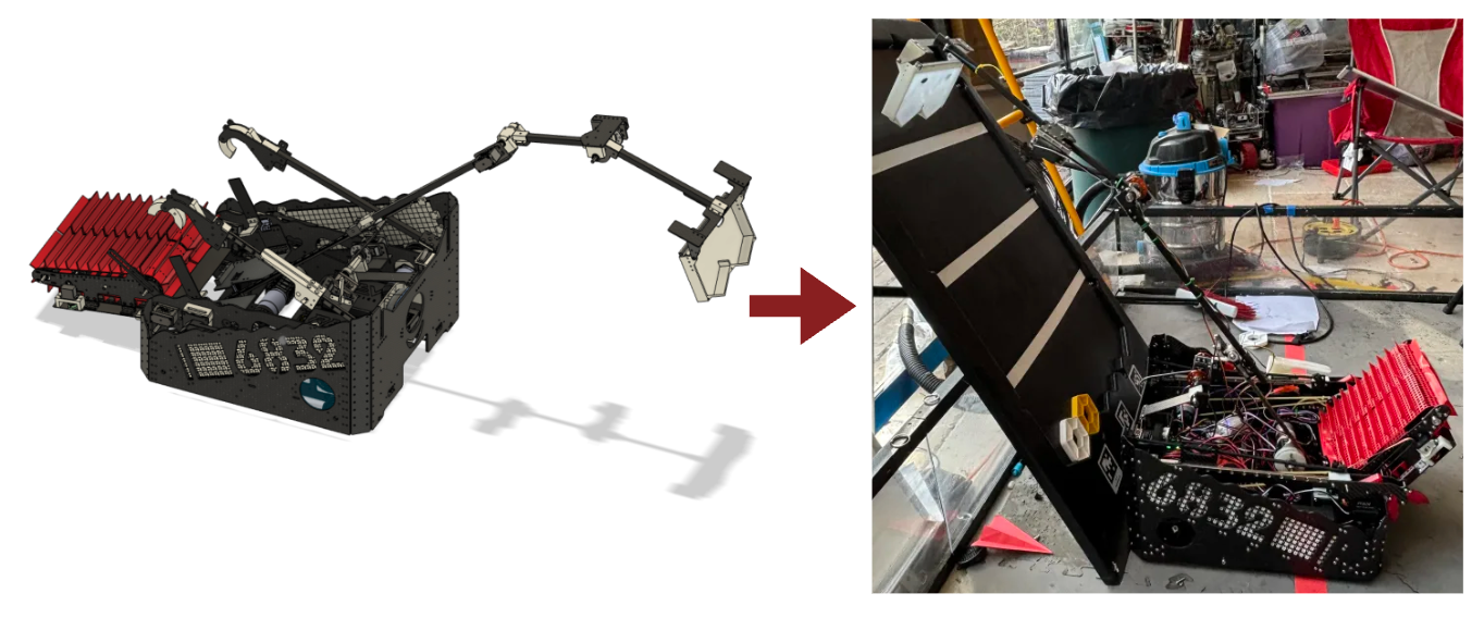
Then, for a quick update on TauBot2, parts of the manufacturing and build have begun, and we hope to incorporate at least part of the new design into the robot we bring to the Tournament on the 28th. Currently, parts of the Chassis and UnderArm have been CNC’ed or 3D printed, and assembly has begun.
Next Steps
Finish up the design of Tau2 and start manufacturing and assembling it, tuning our autonomous and anti-tipping code, and attempting to get more driver practice in preparation for next week’s Tournament.
 Match 7(Q121)


 Finals 2
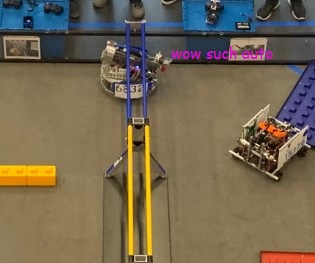


 Finals 2


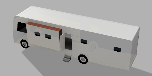


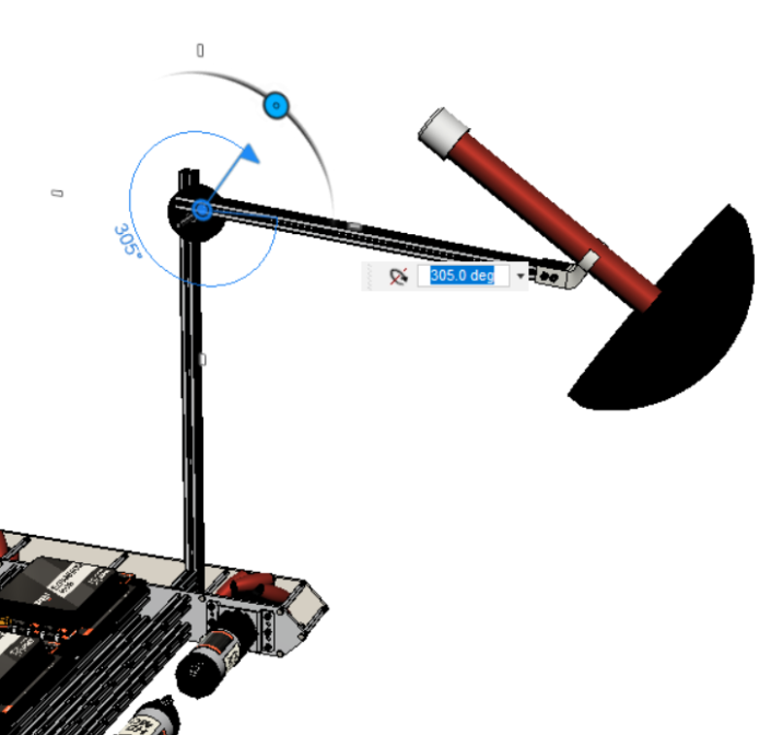
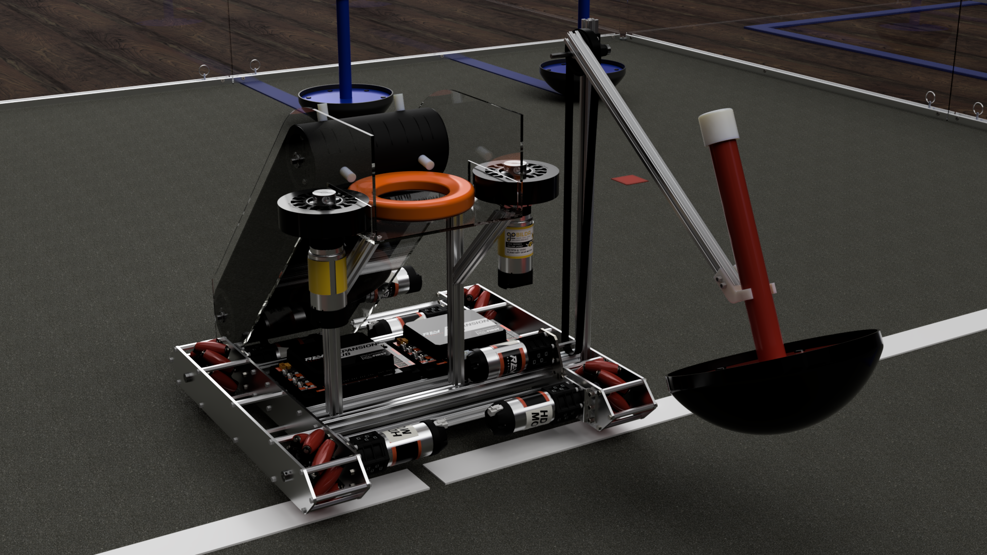
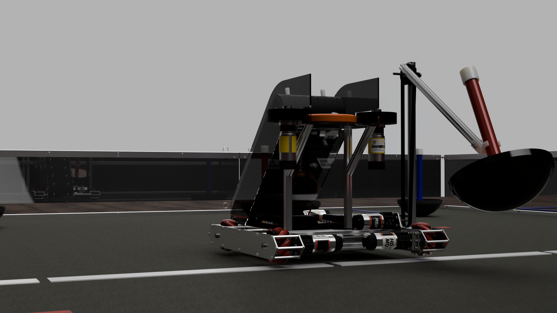
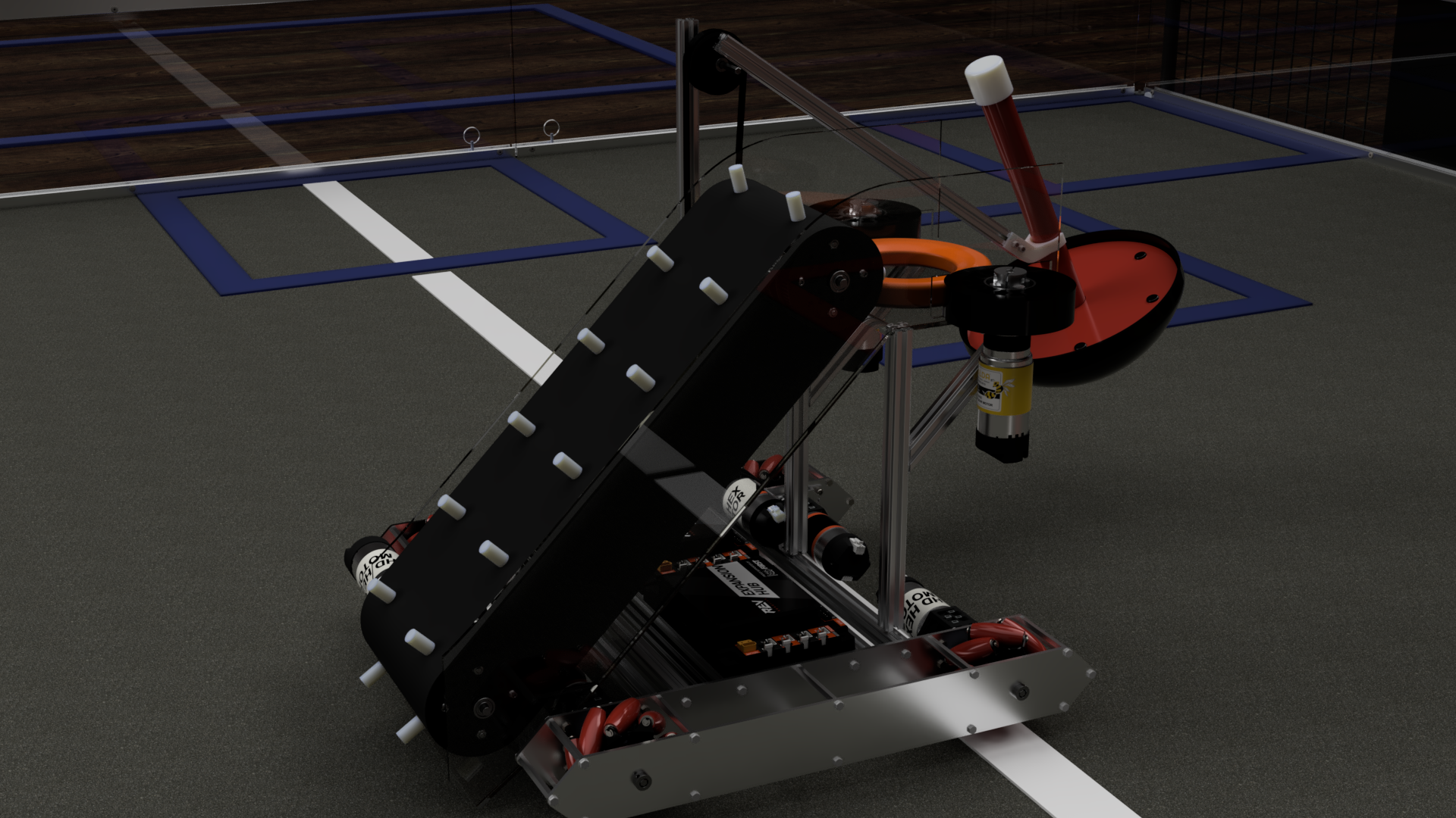

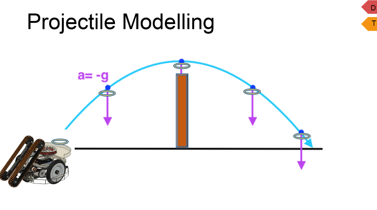
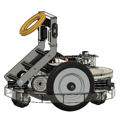


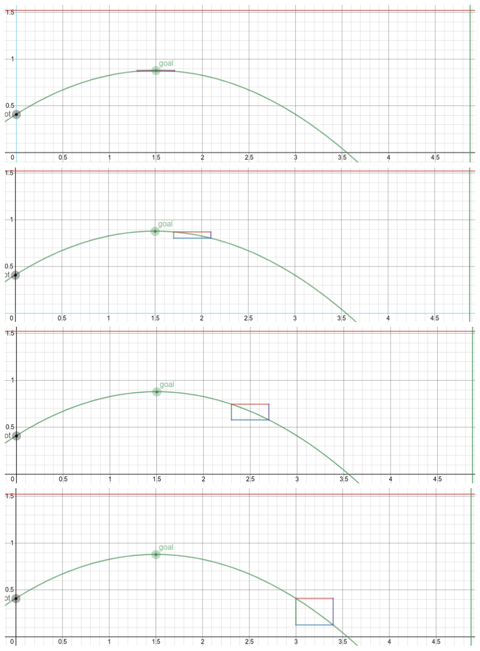


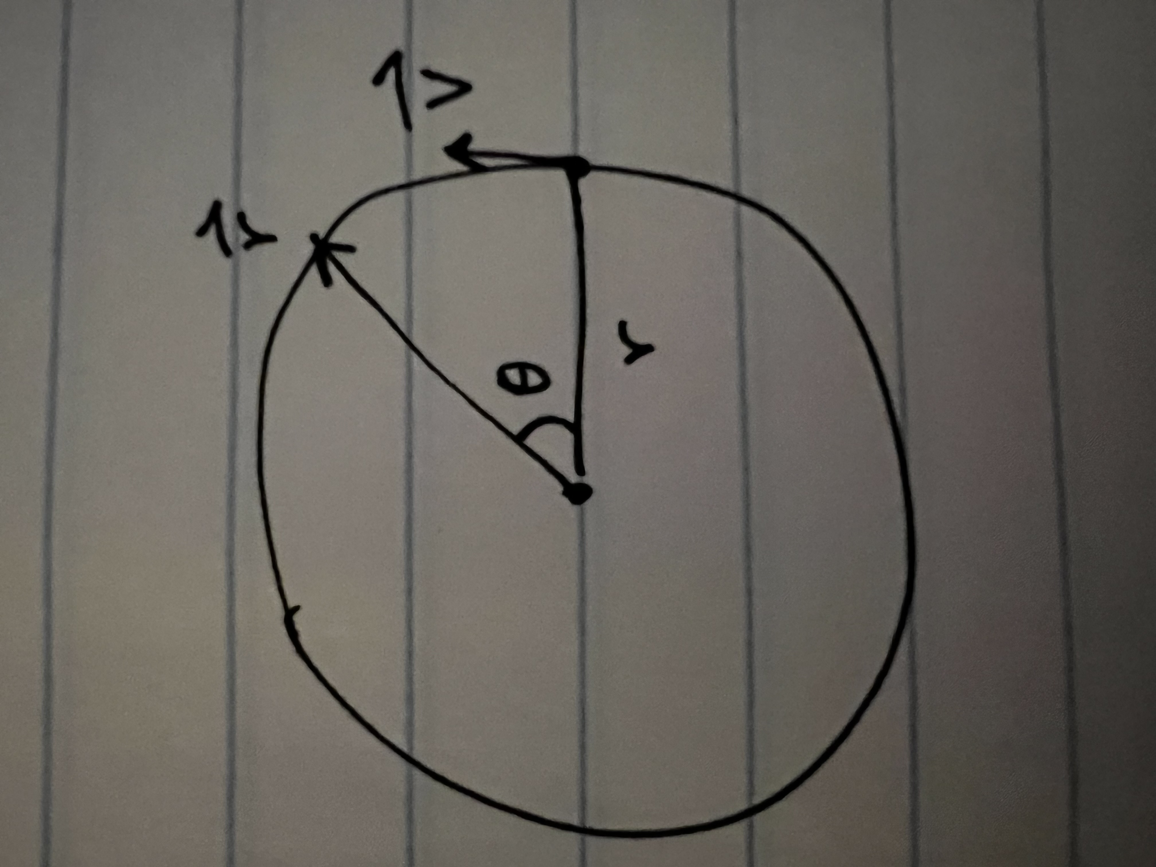
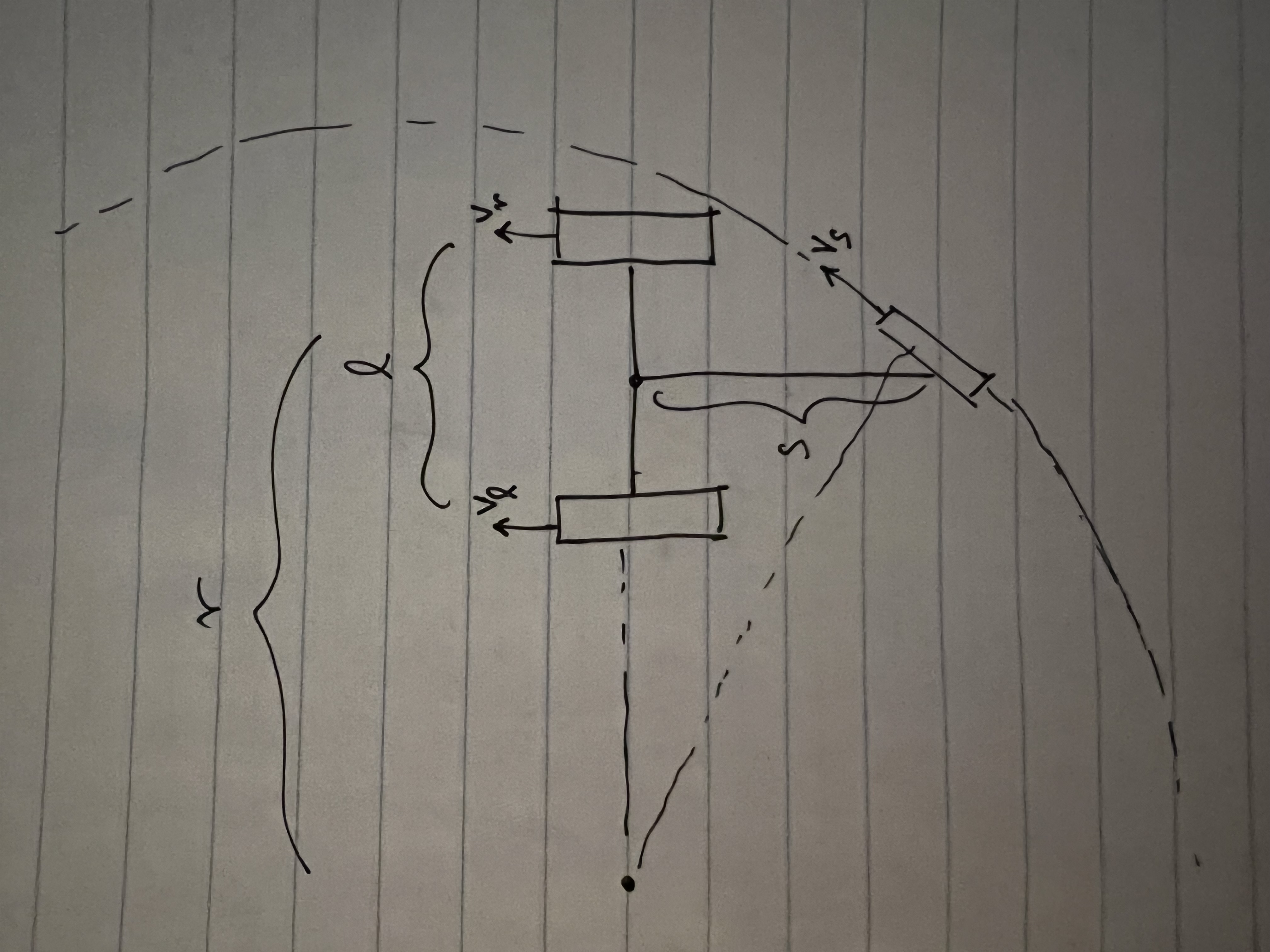
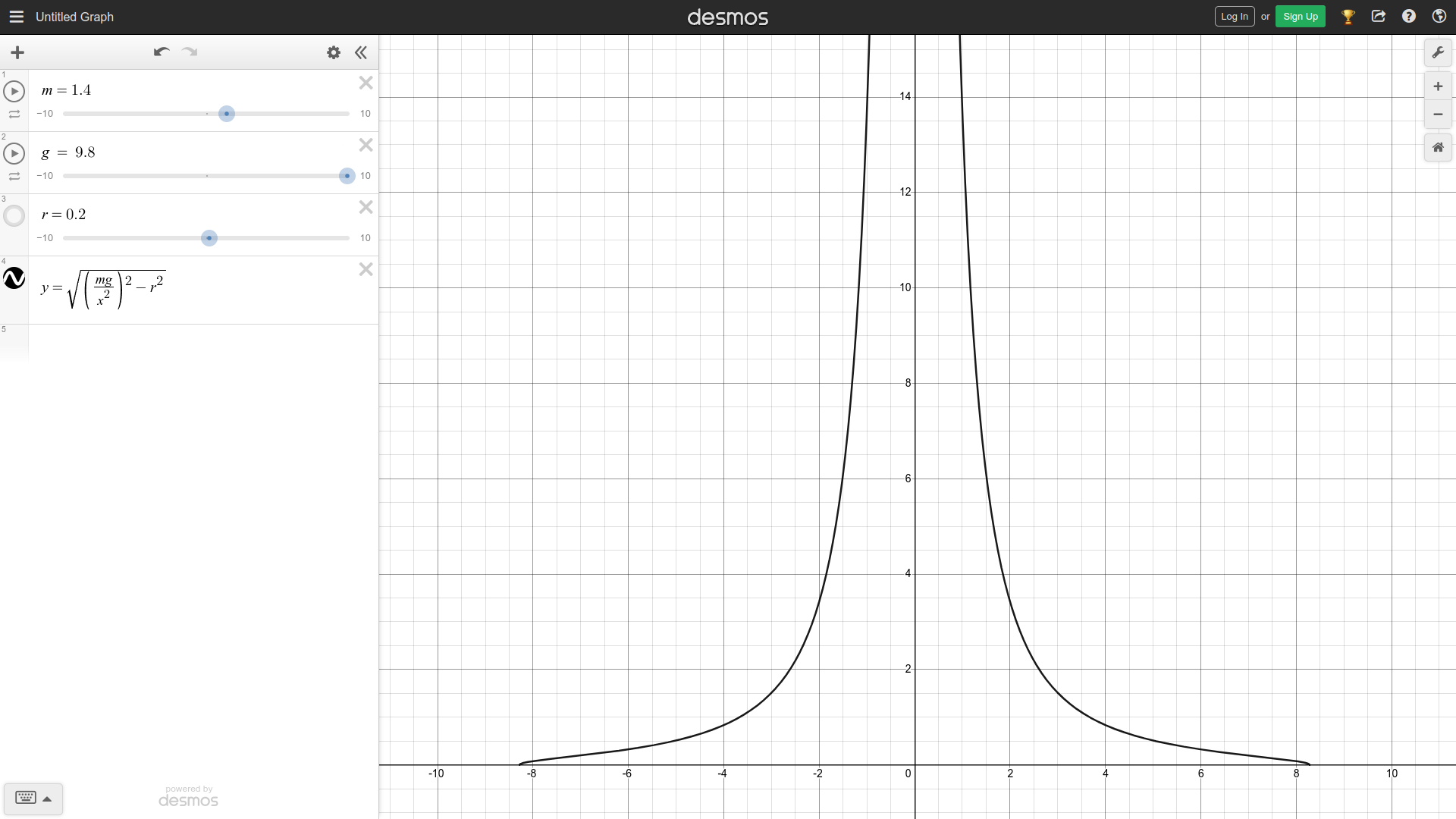
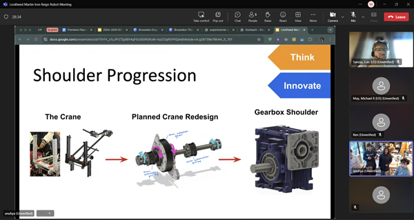
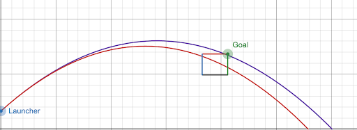
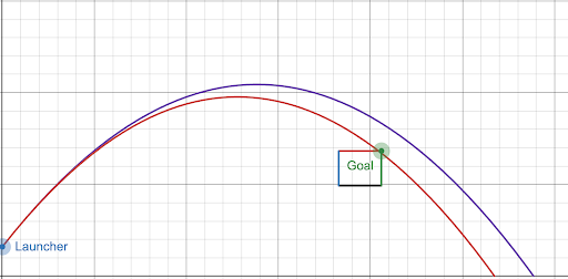
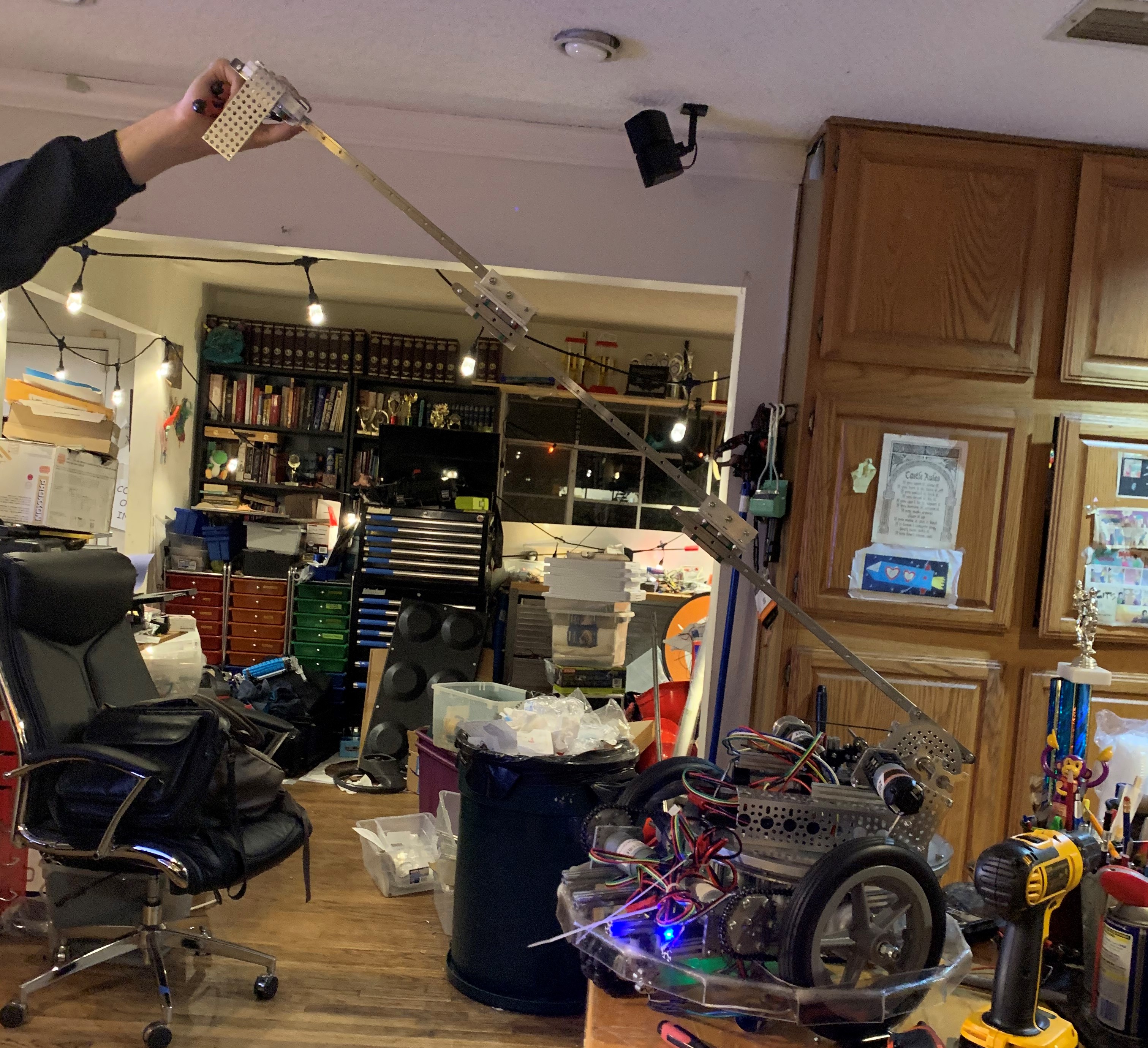
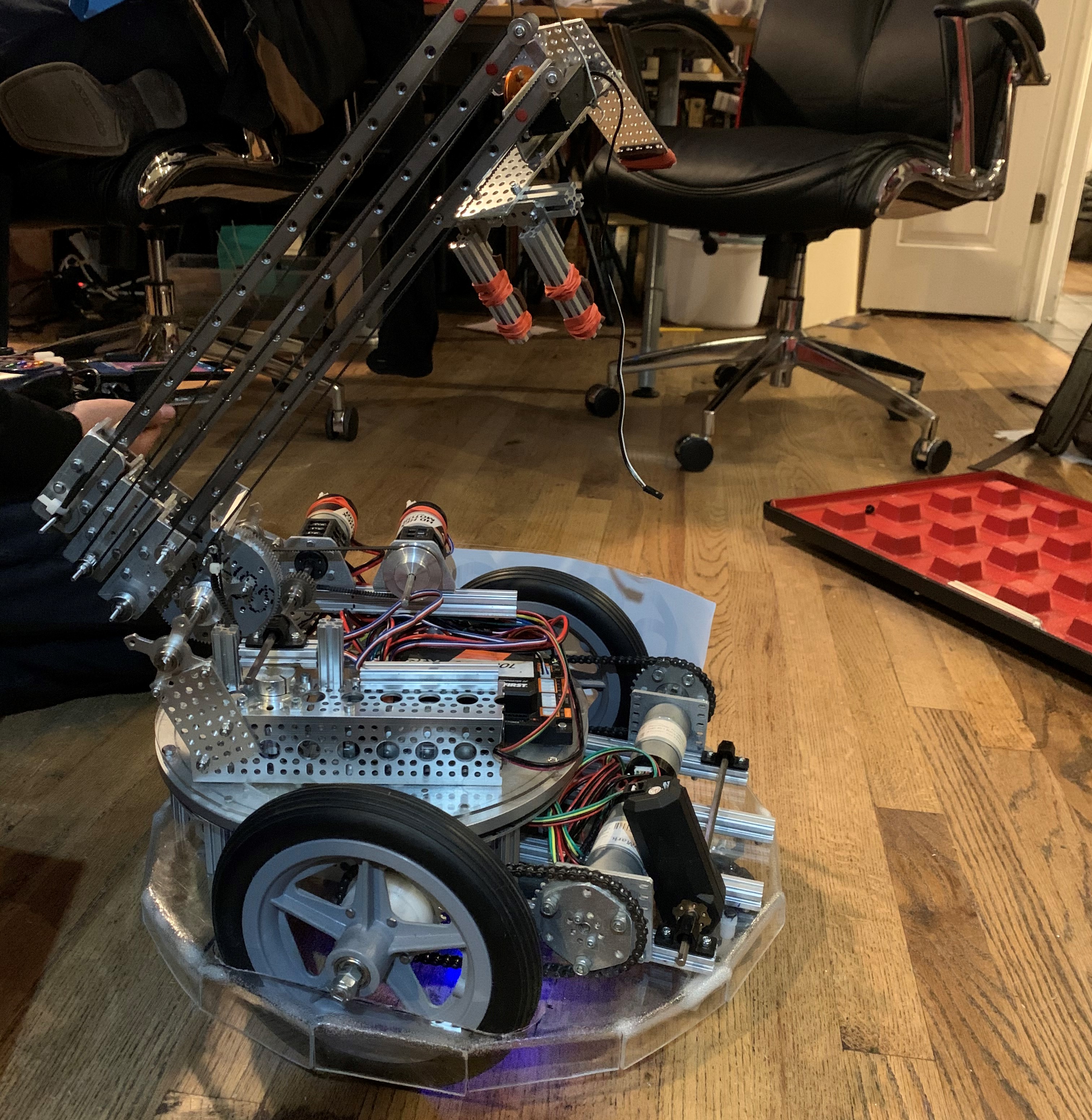
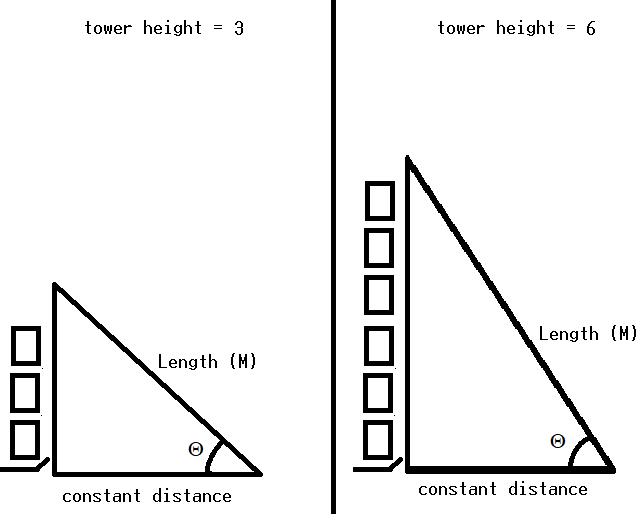
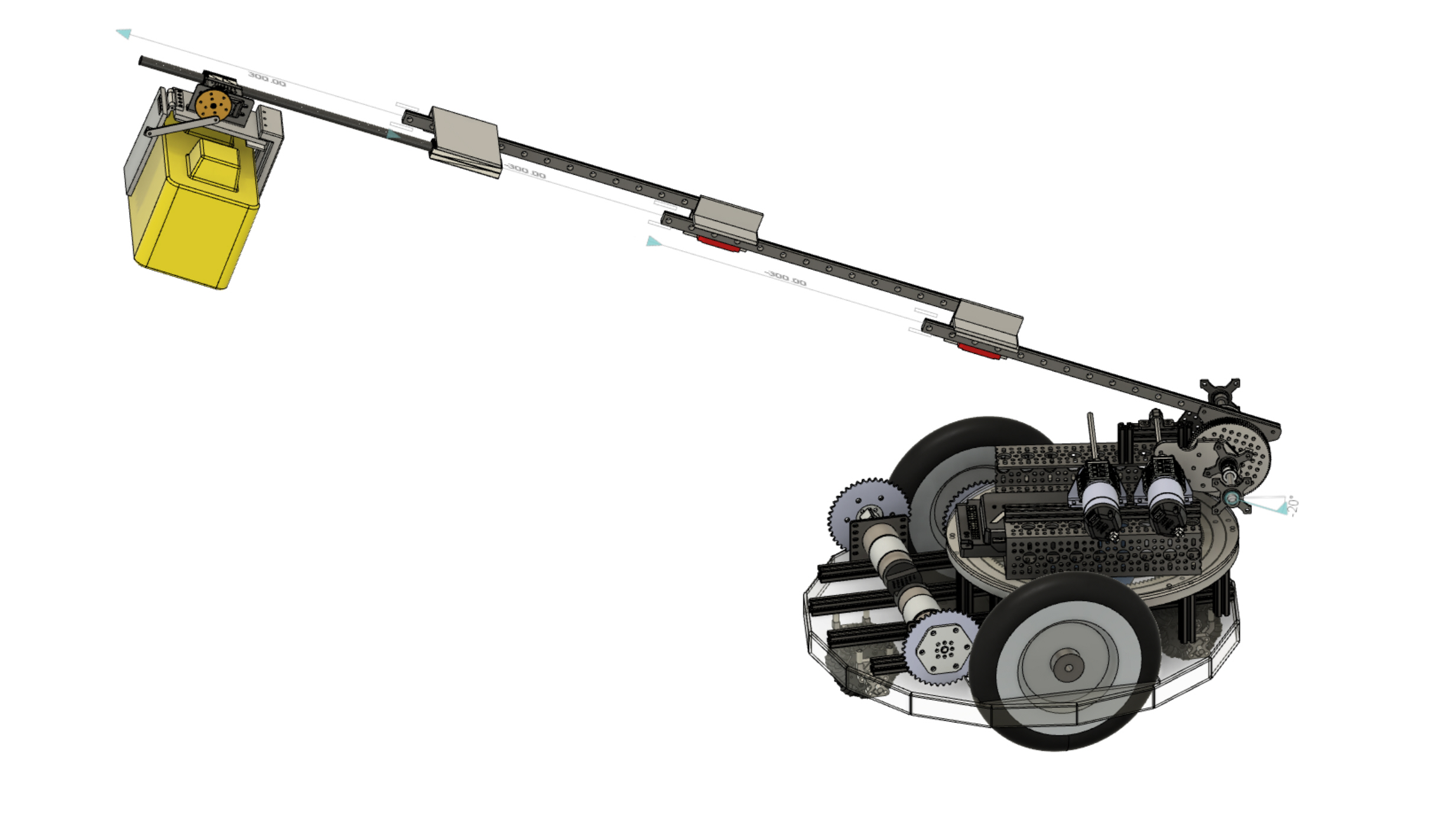
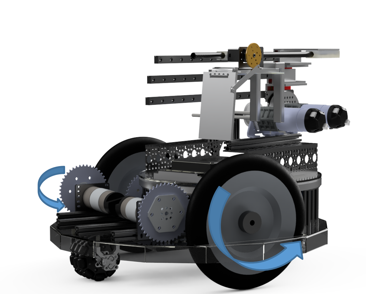
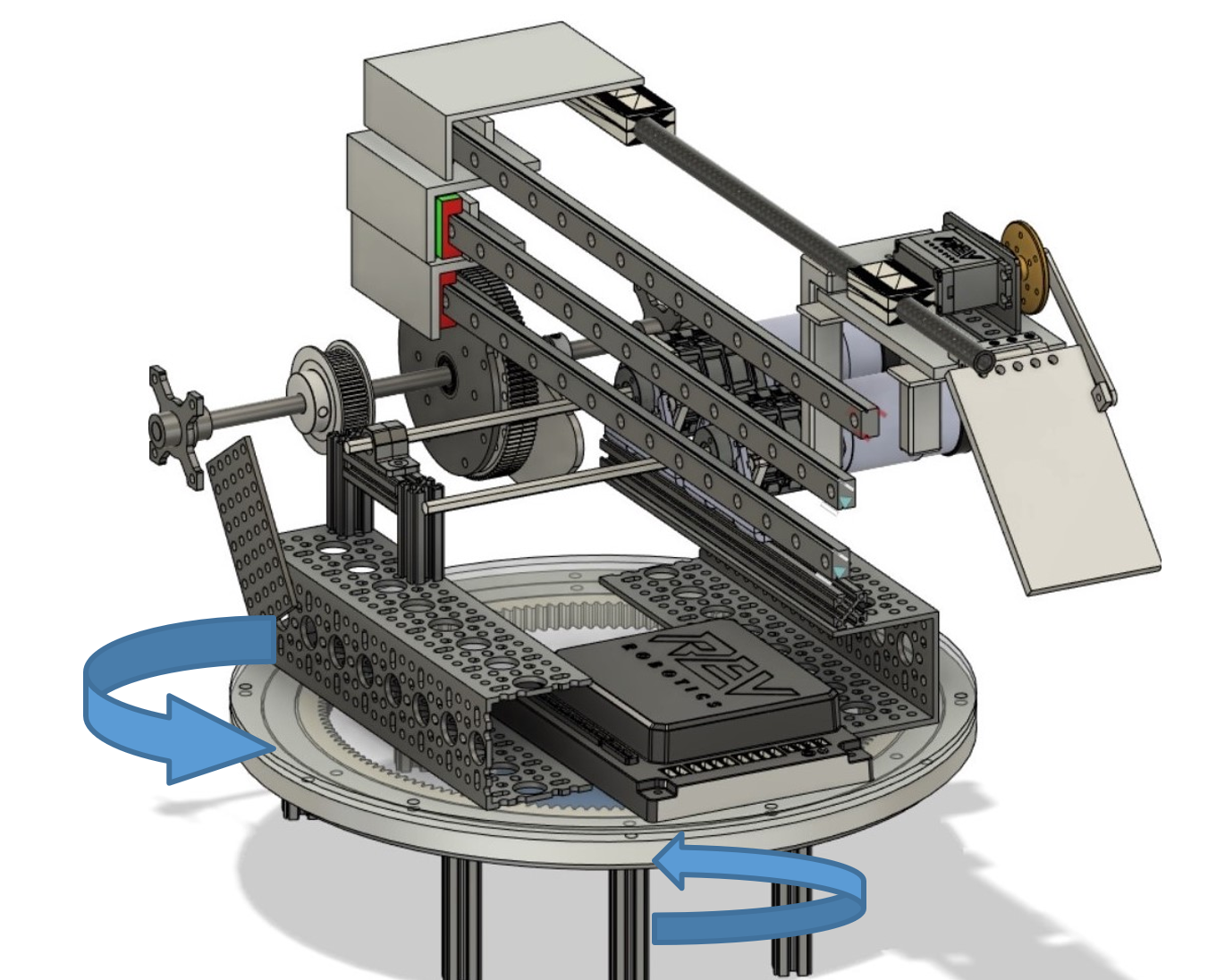
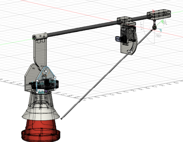
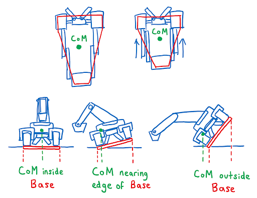 Looking at these diagrams of the robot and its center of mass, we can see how as the crane extends past the base of the robot, the center of mass moves towards the base. Eventually, the center of mass reaches a position outside of the base and the robot falls over. To solve this problem, we would have to either lower the center of mass or limit its fluctuation during movement.
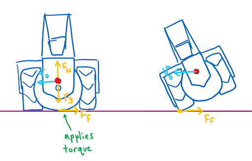
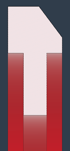
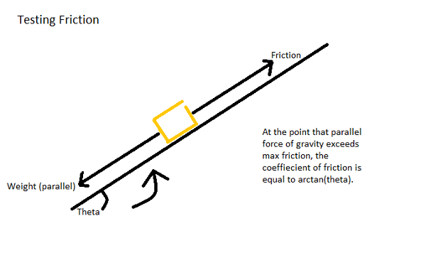
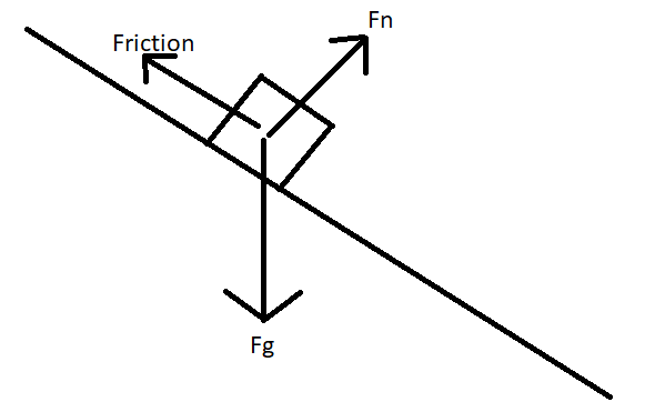
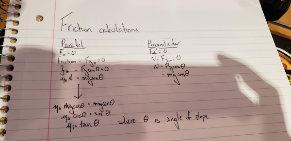
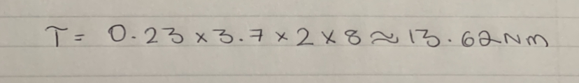
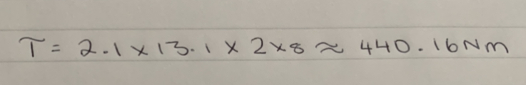
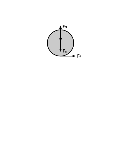 You can see from these free-body diagrams that as we lower the vertical component of the normal force, the overall rotational torque exerted by the swerve module is decreased, which inspired our decisions to lower the center of mass.
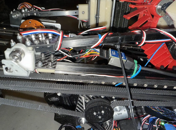
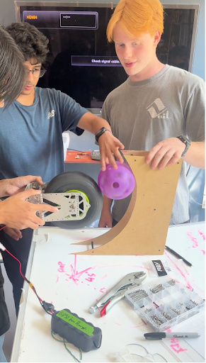
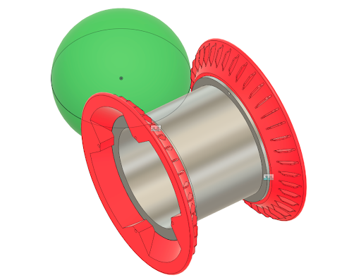
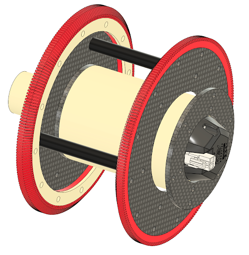
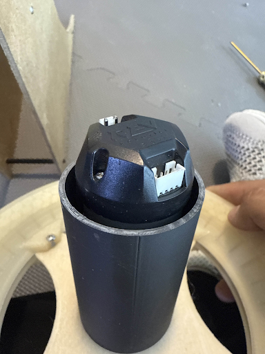
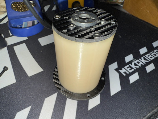
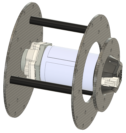
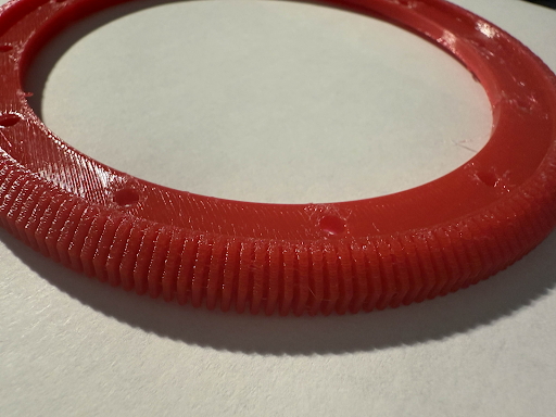
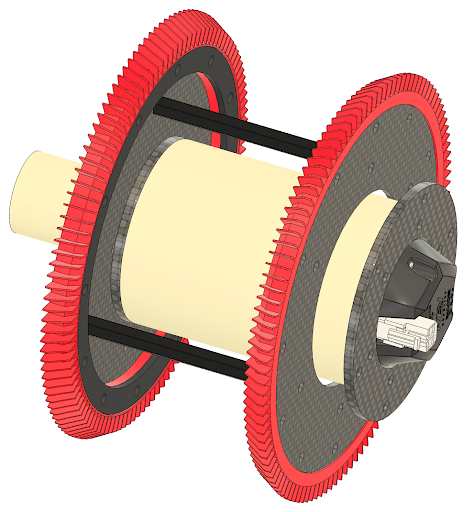
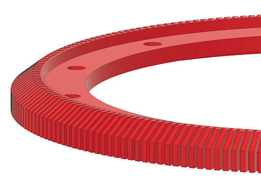
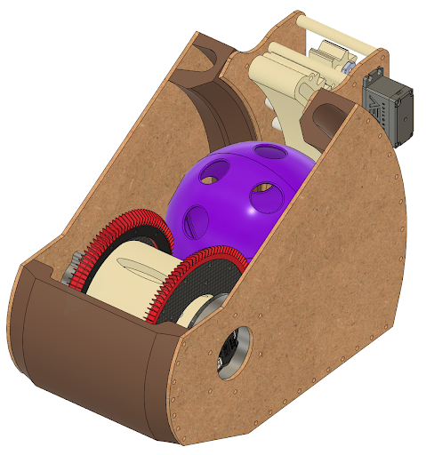
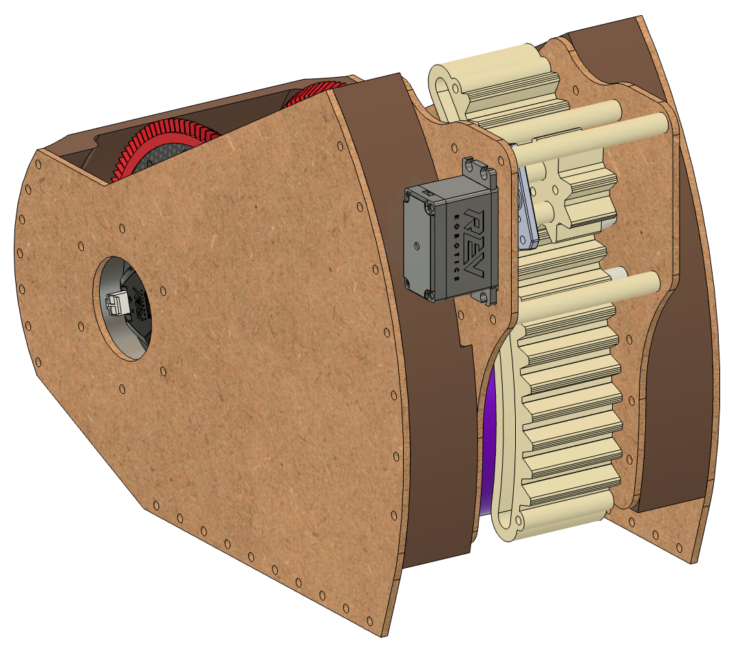
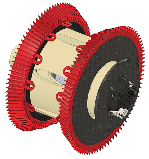
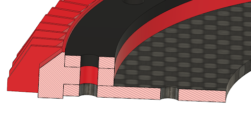
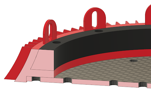
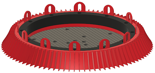
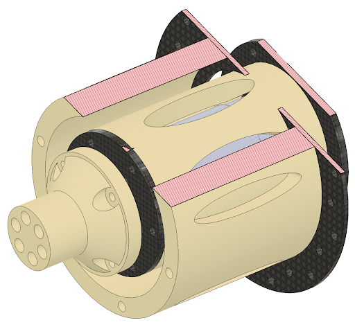
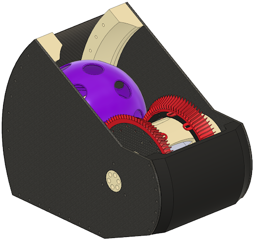
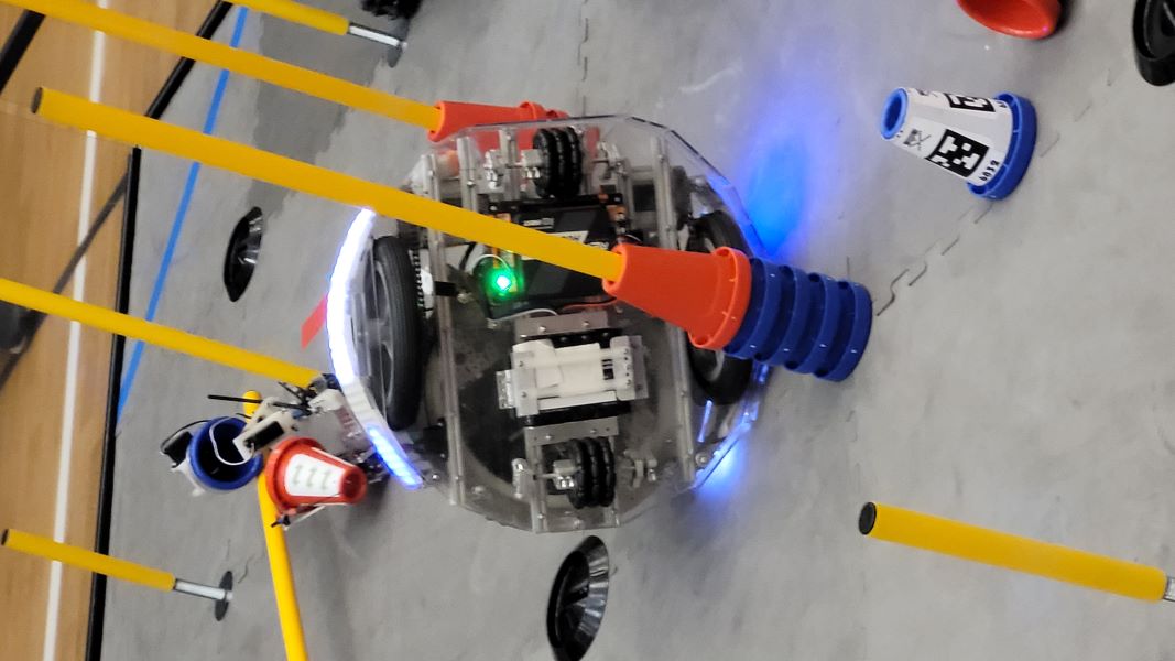
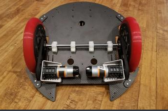
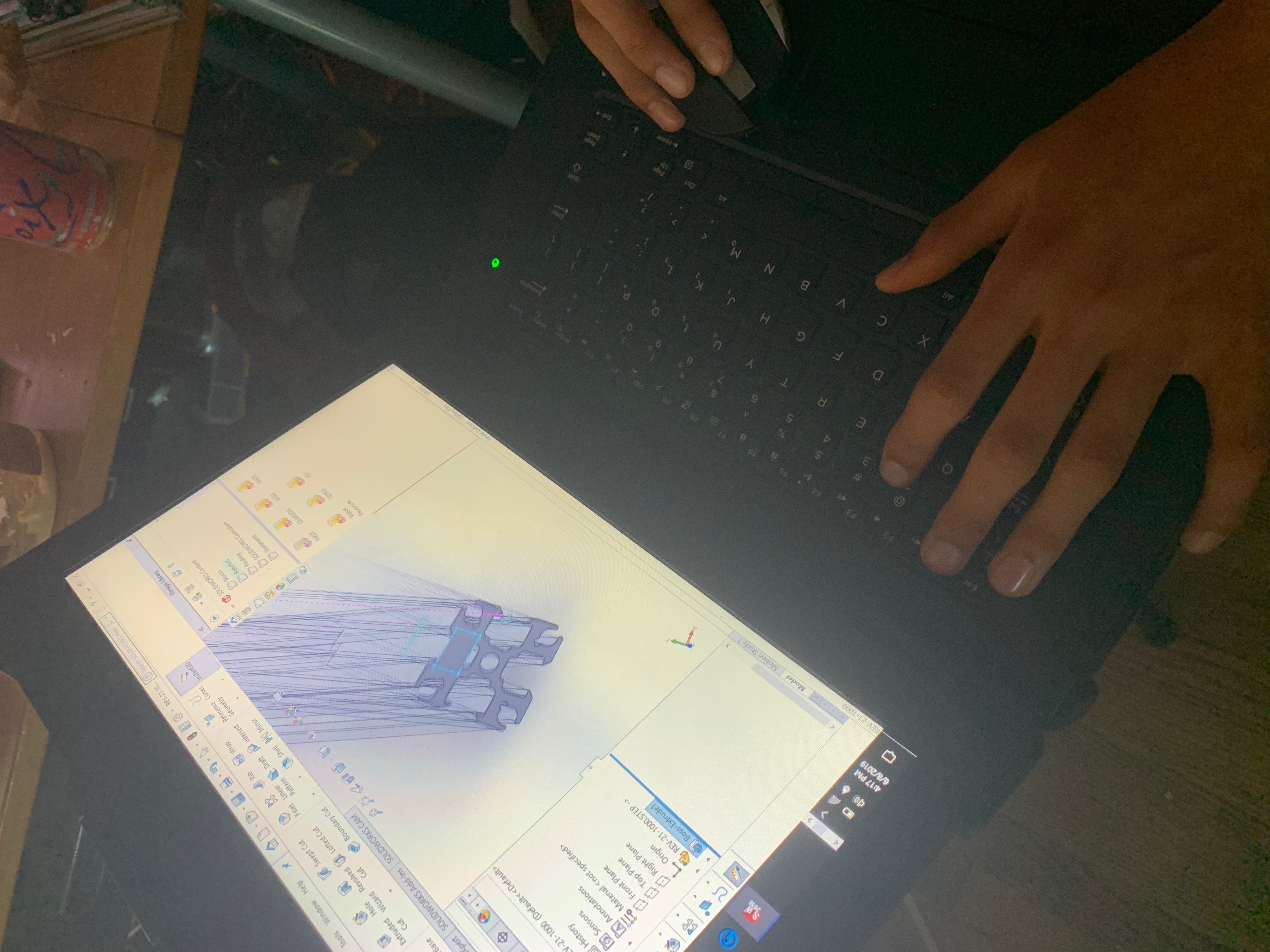
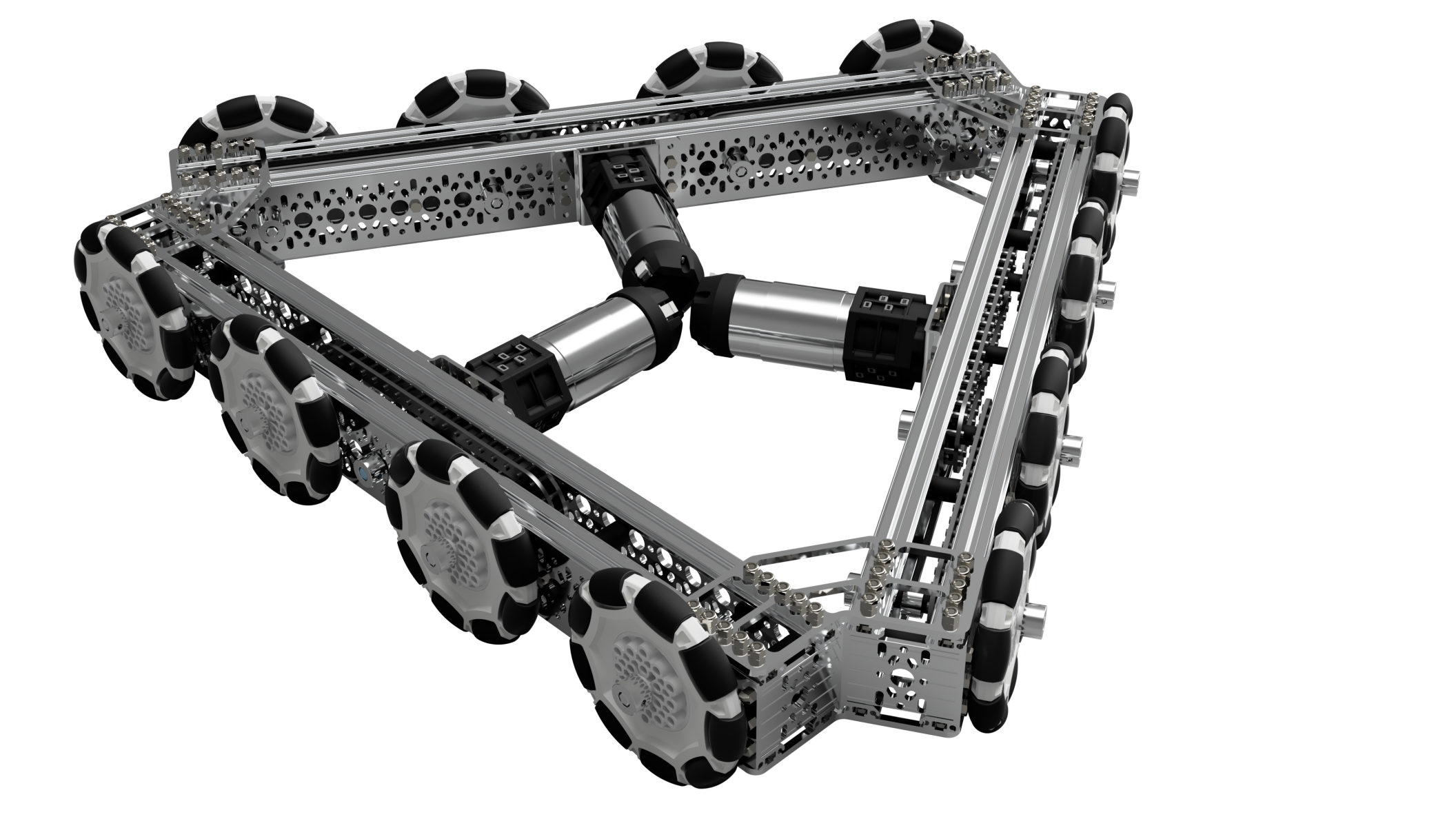
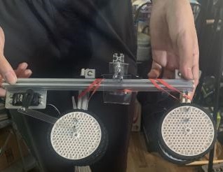
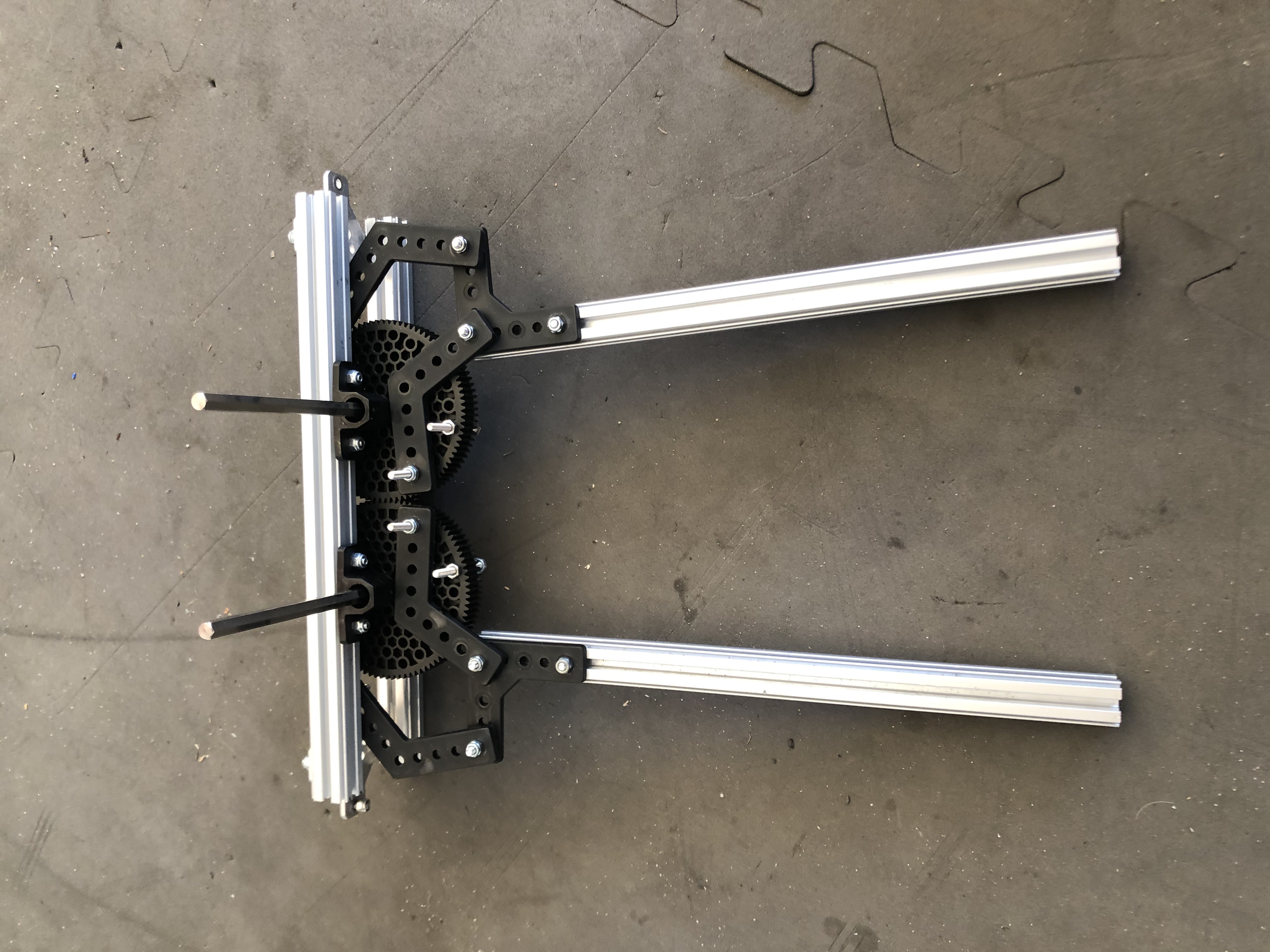
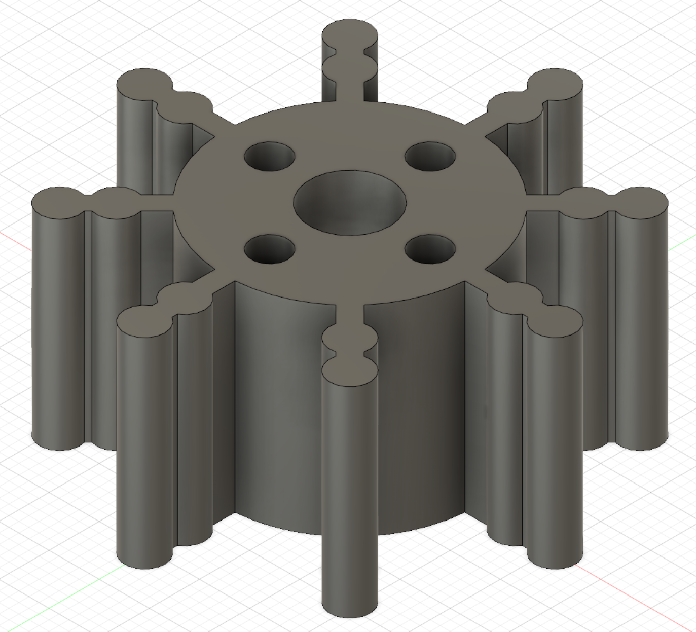
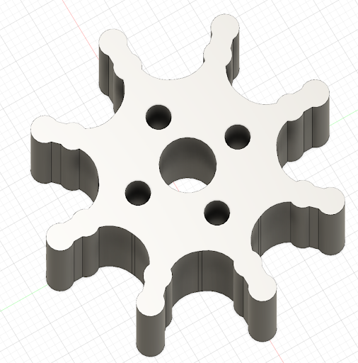
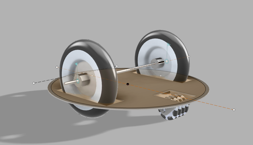
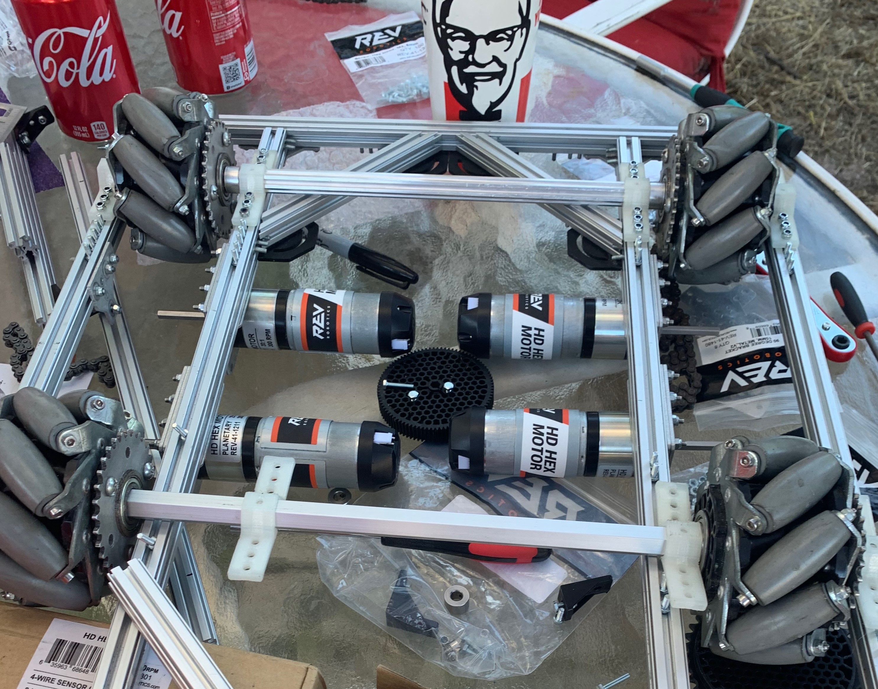
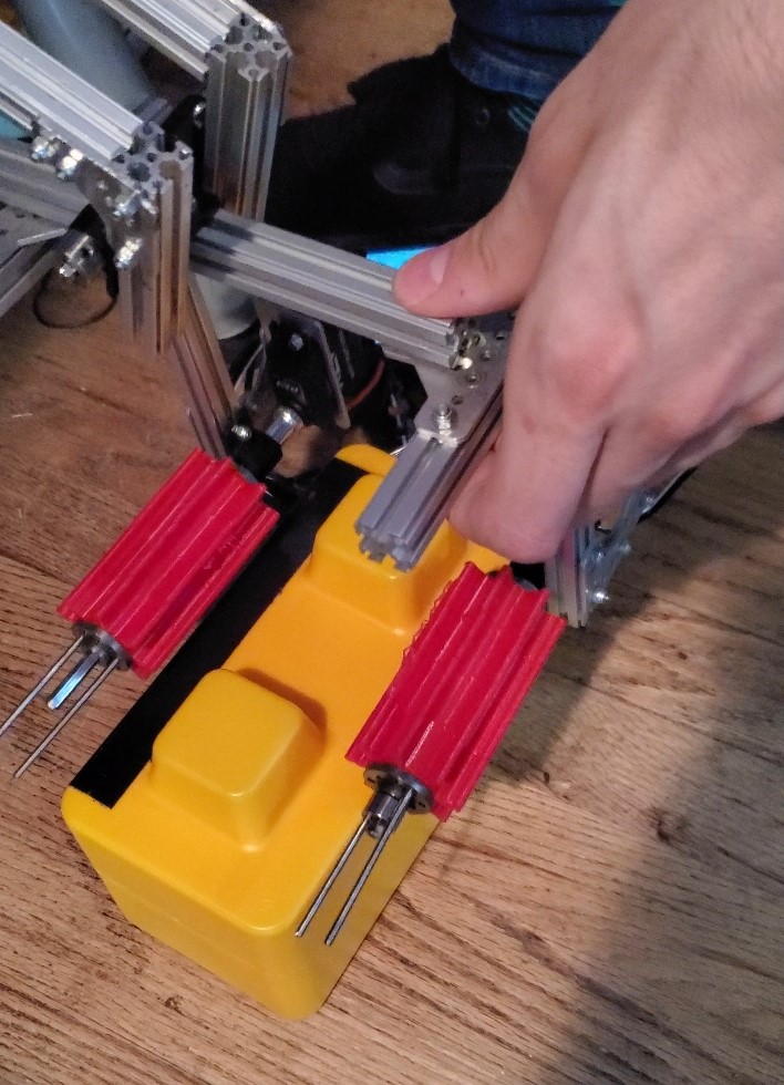
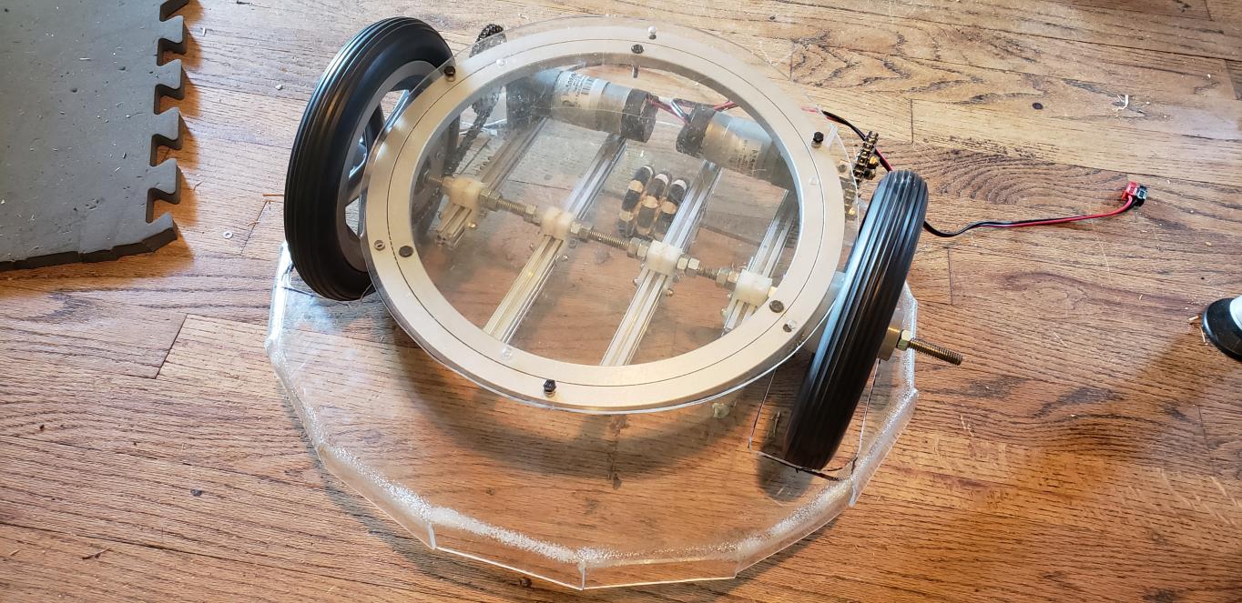
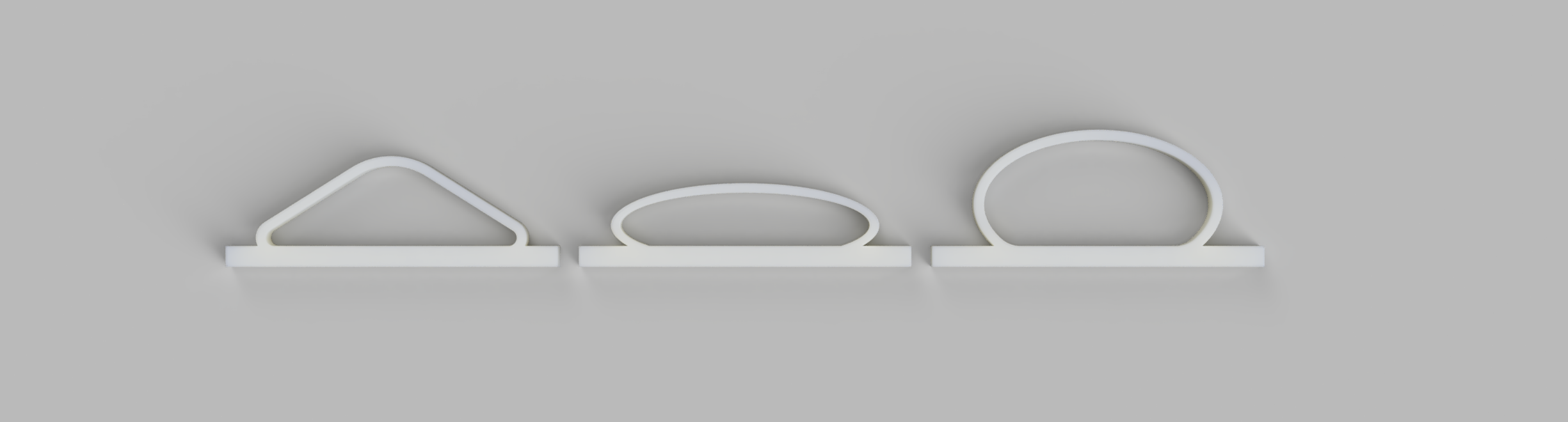
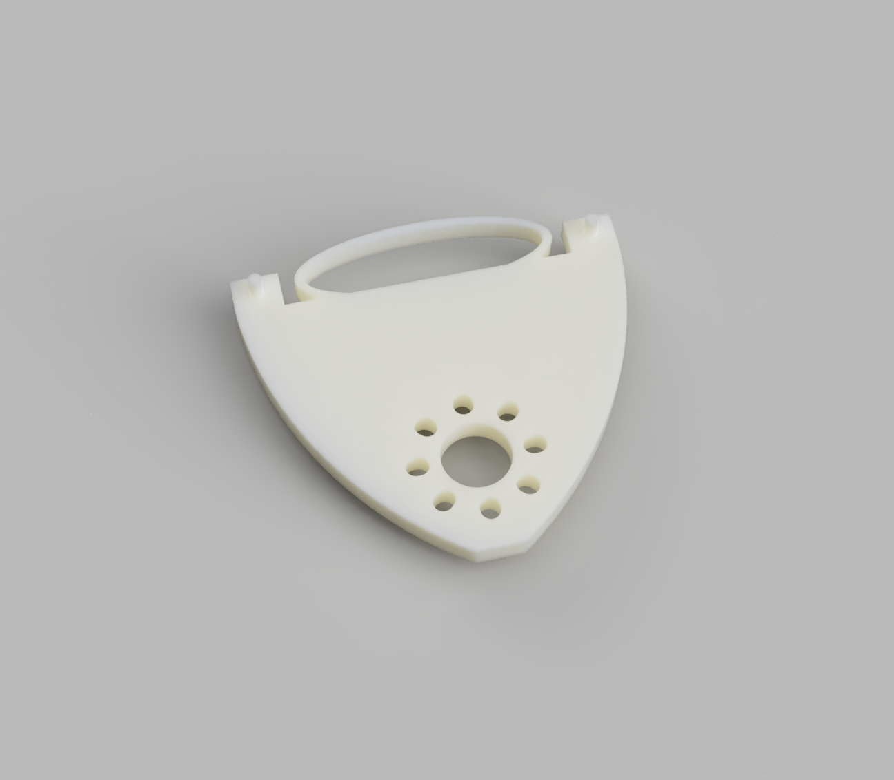
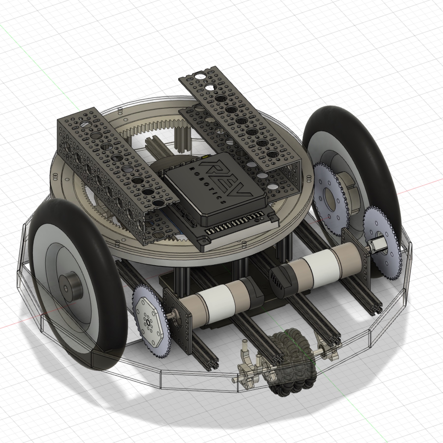
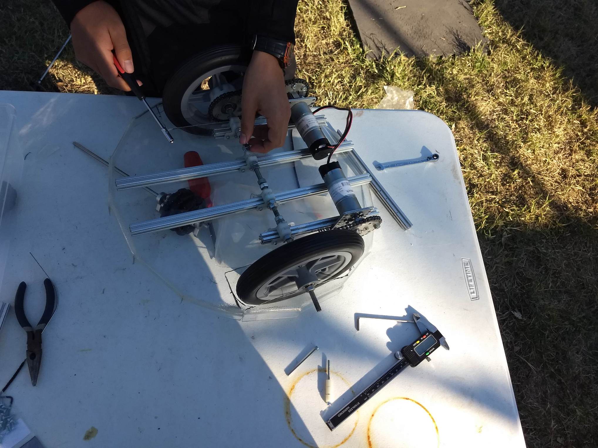
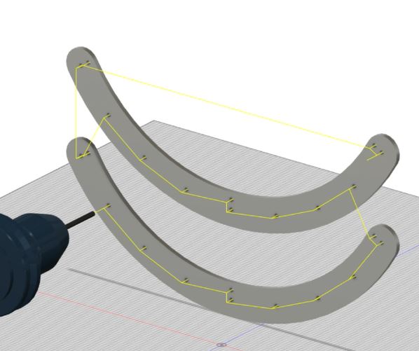
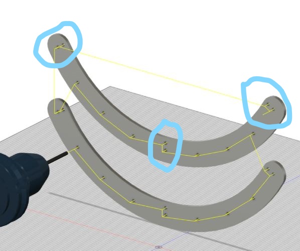
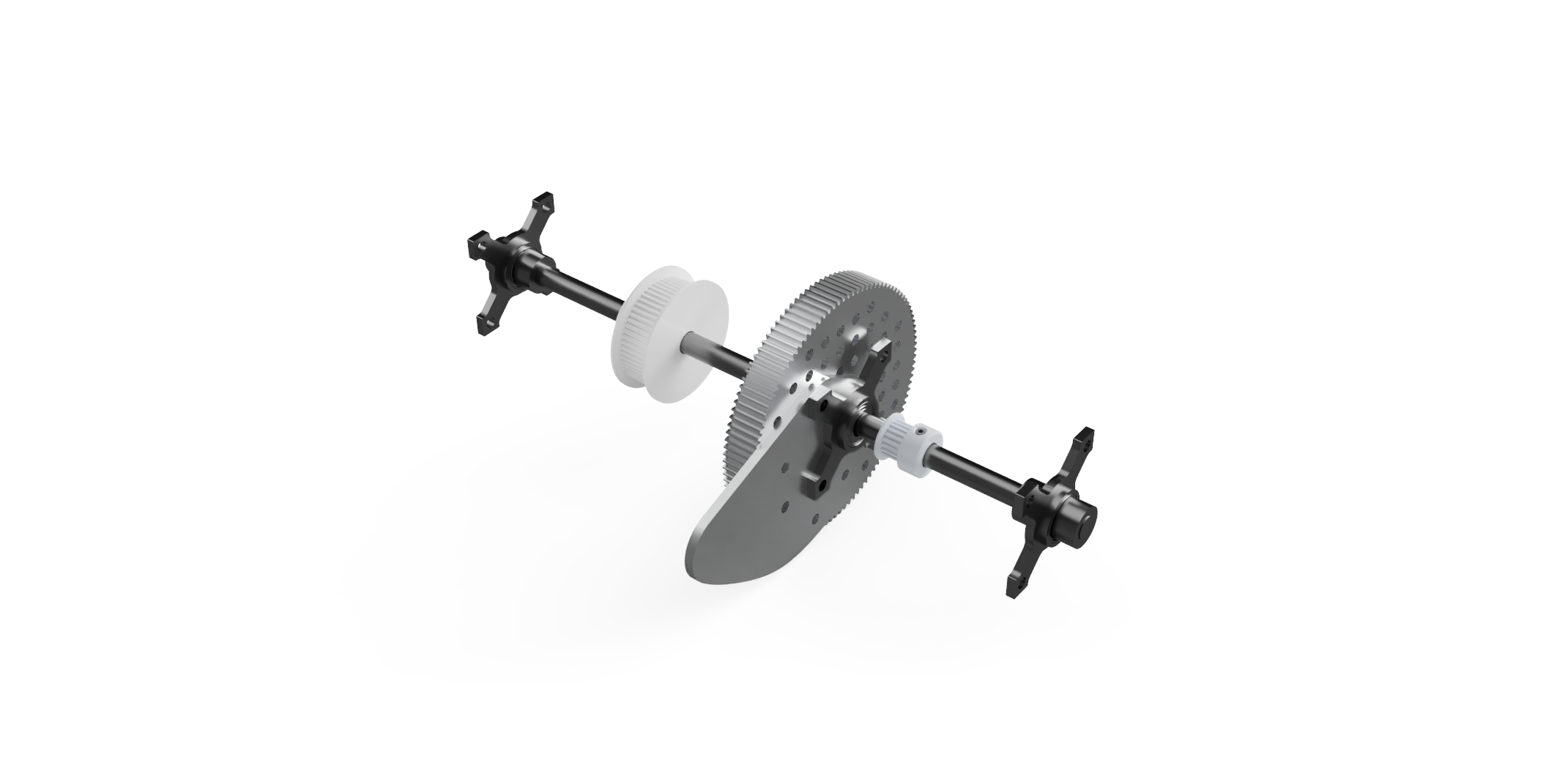
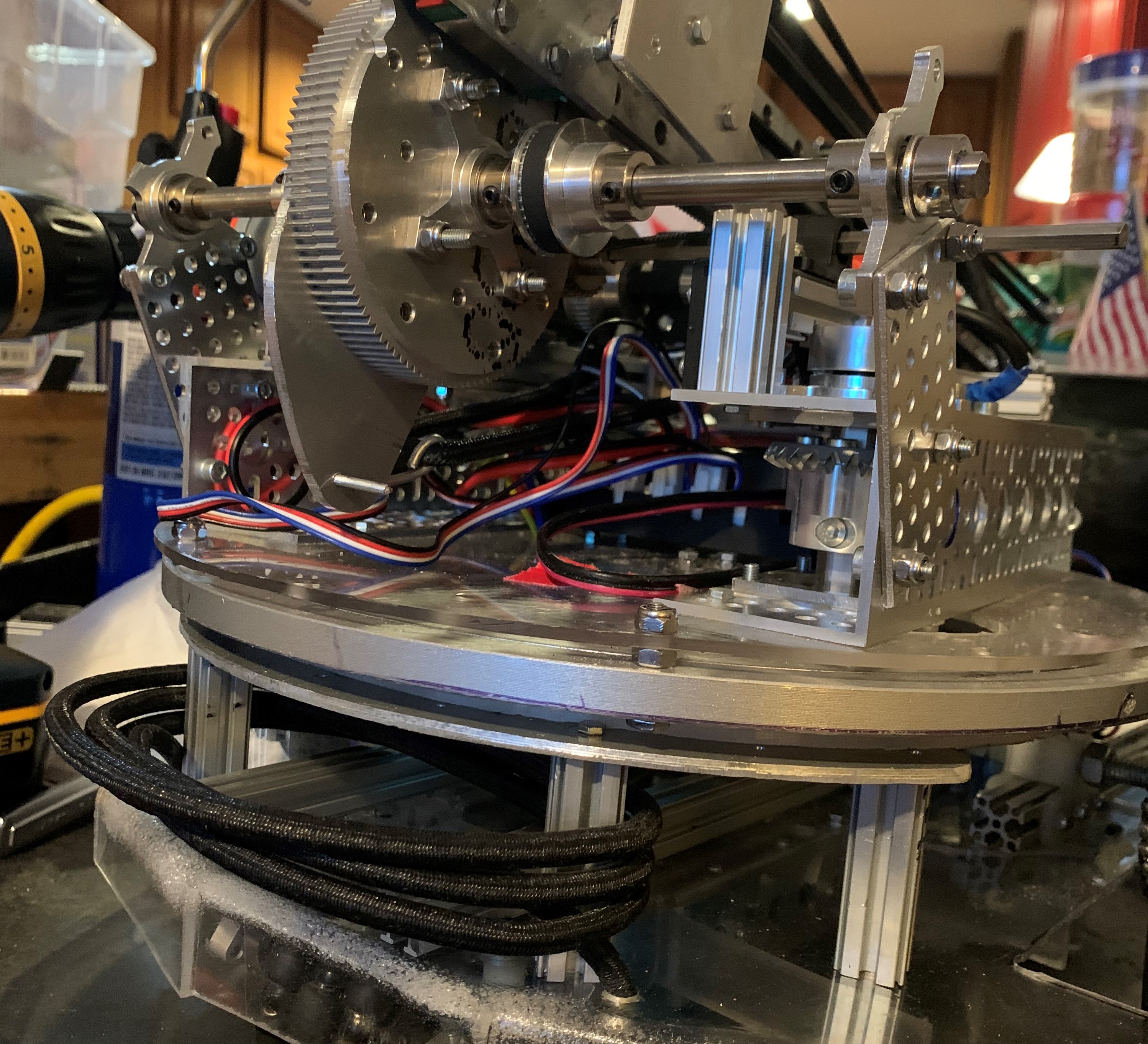
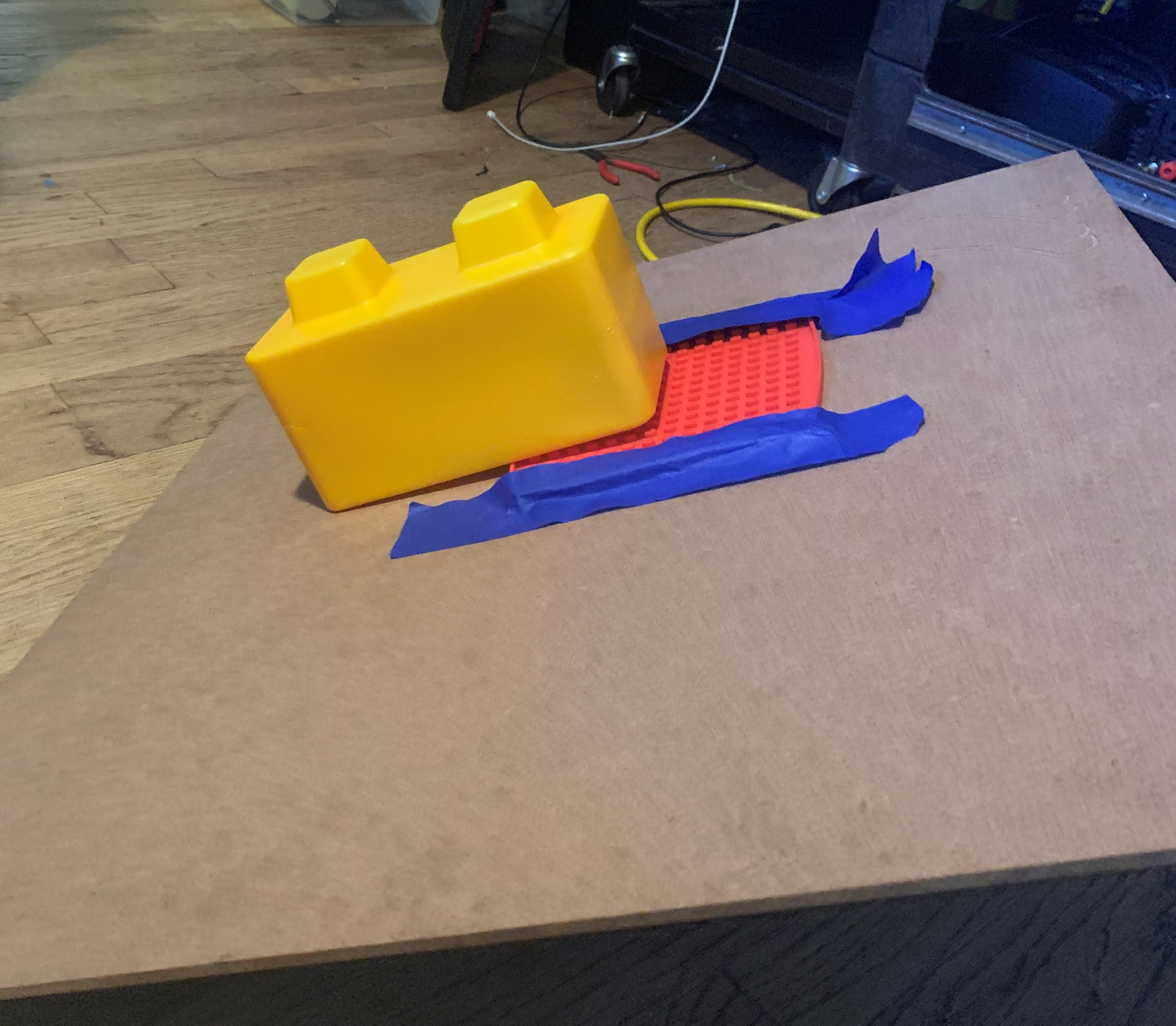
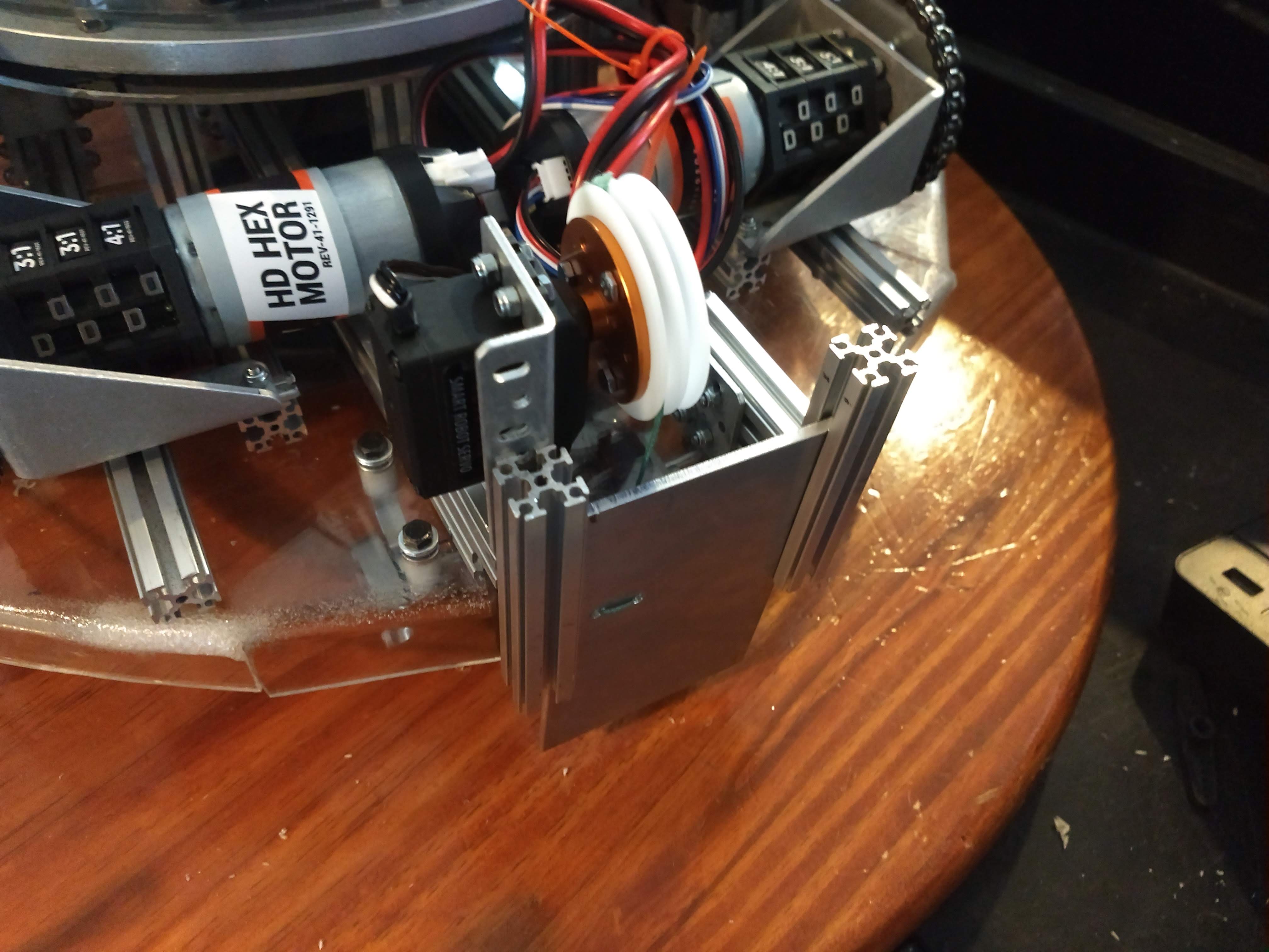
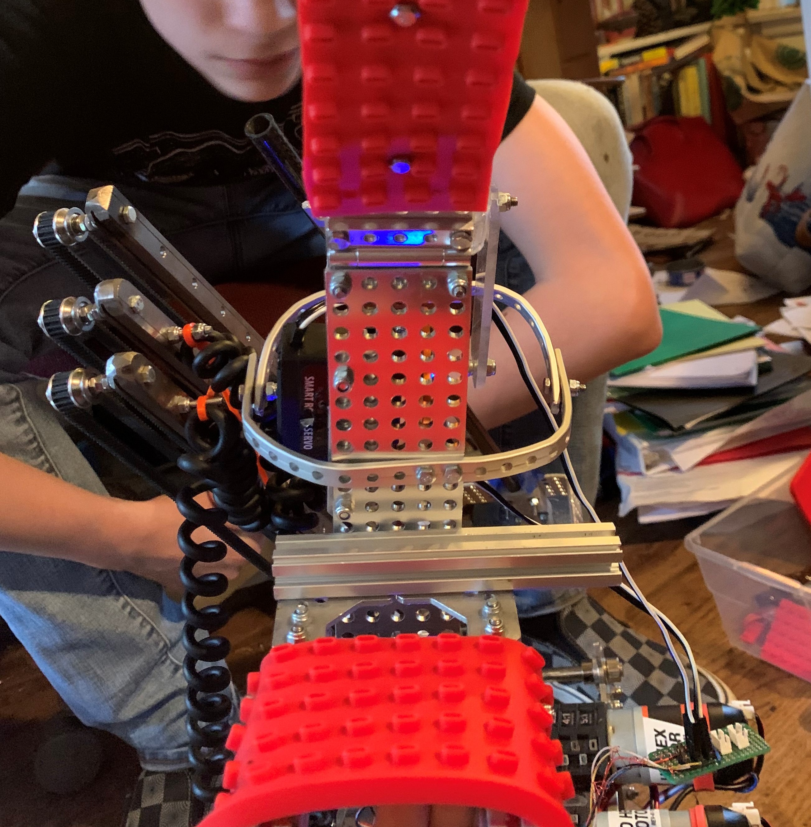
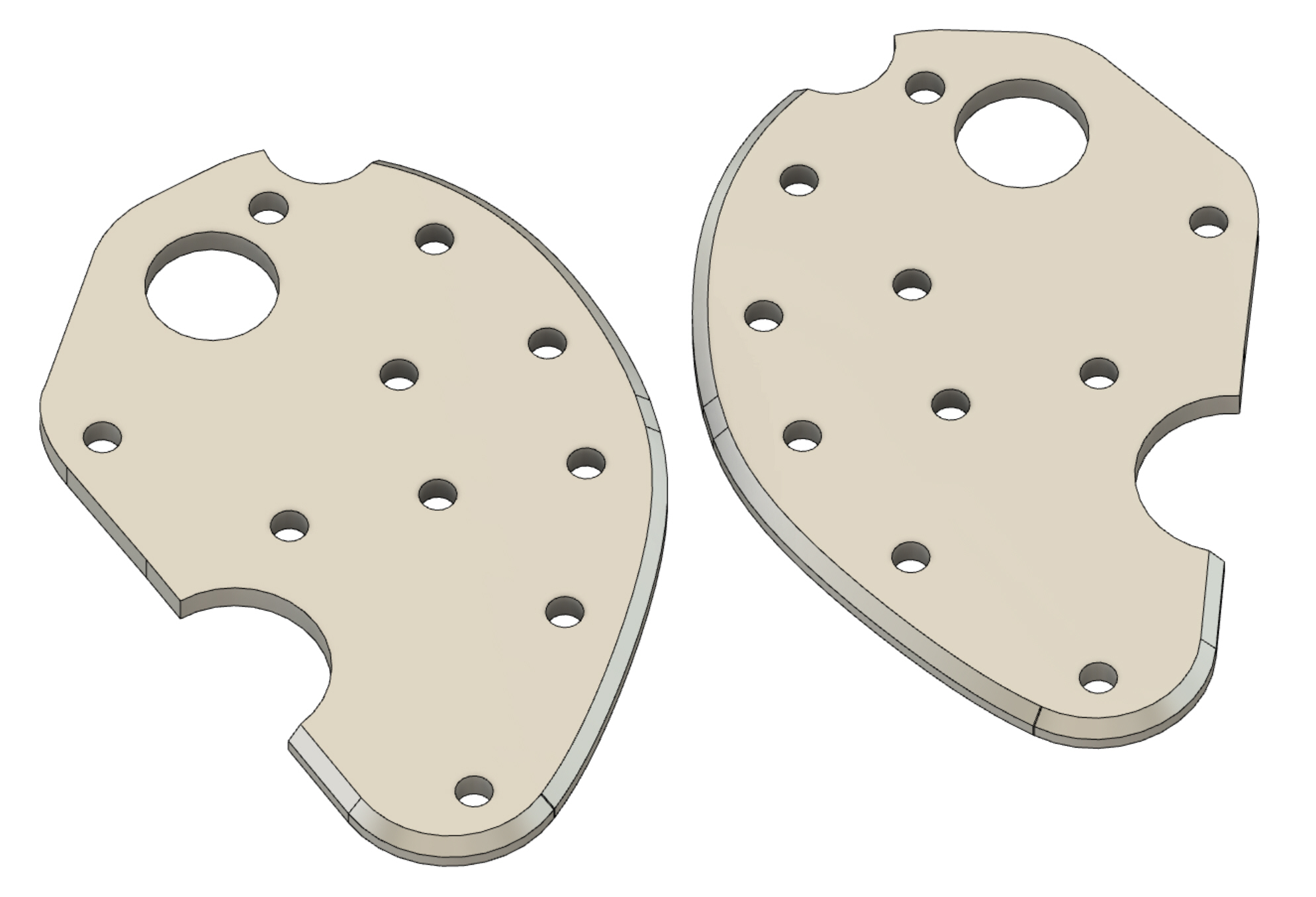
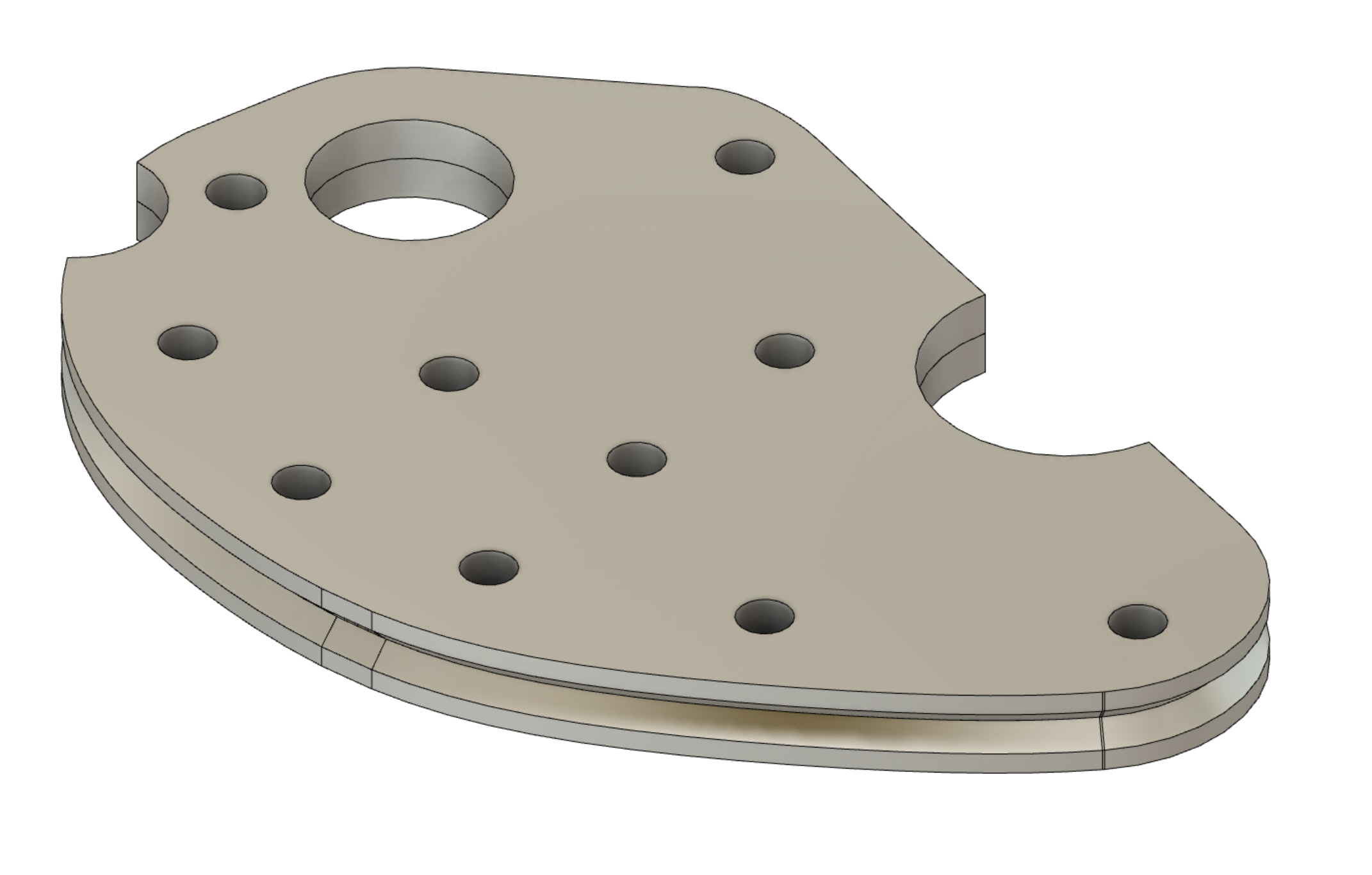
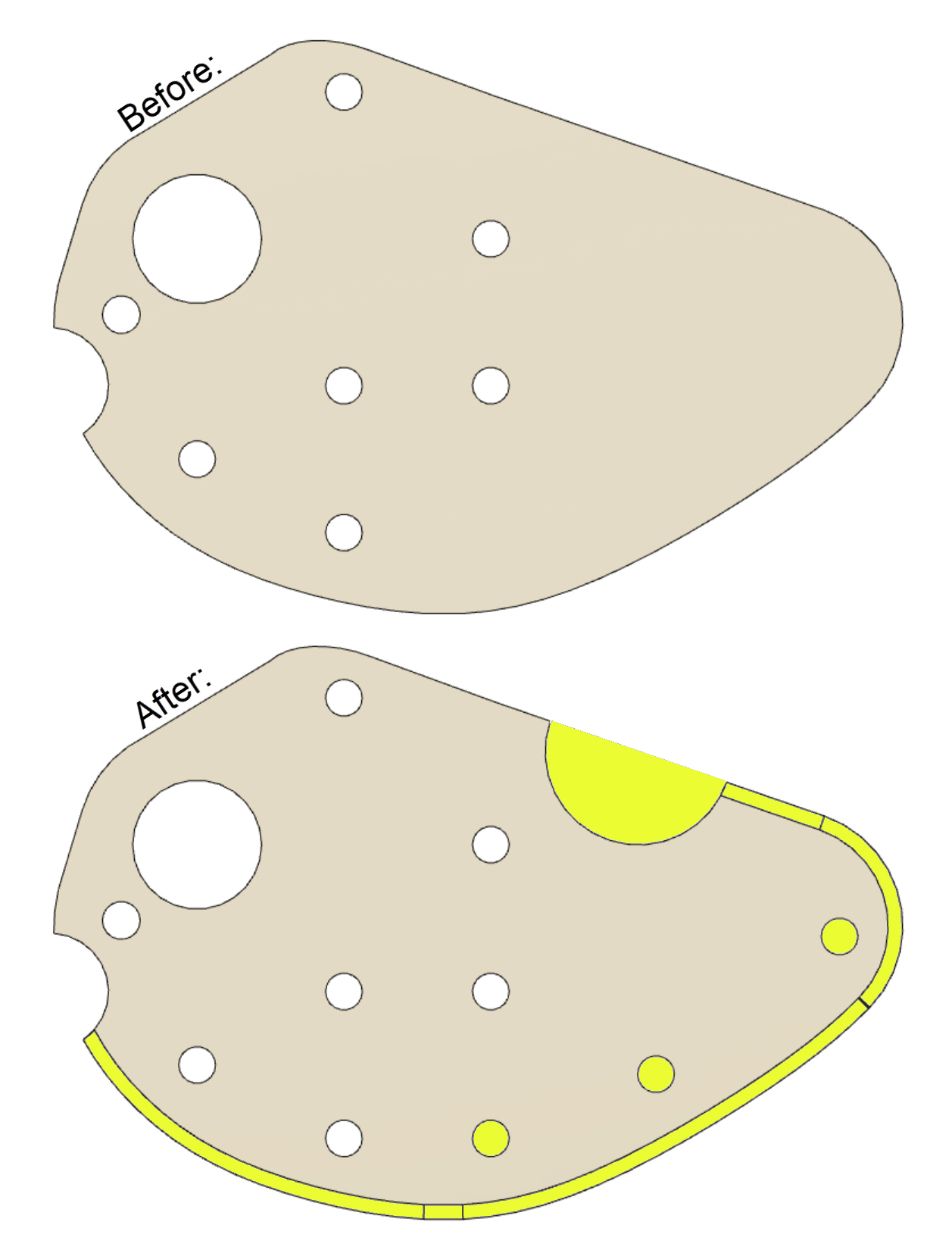
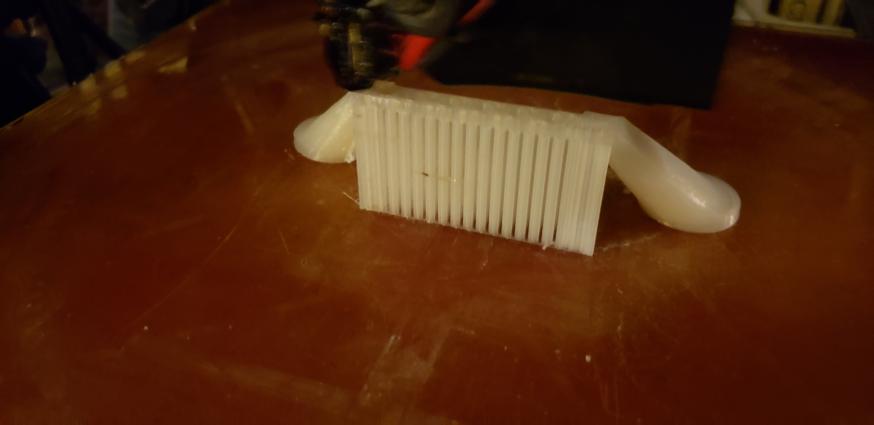
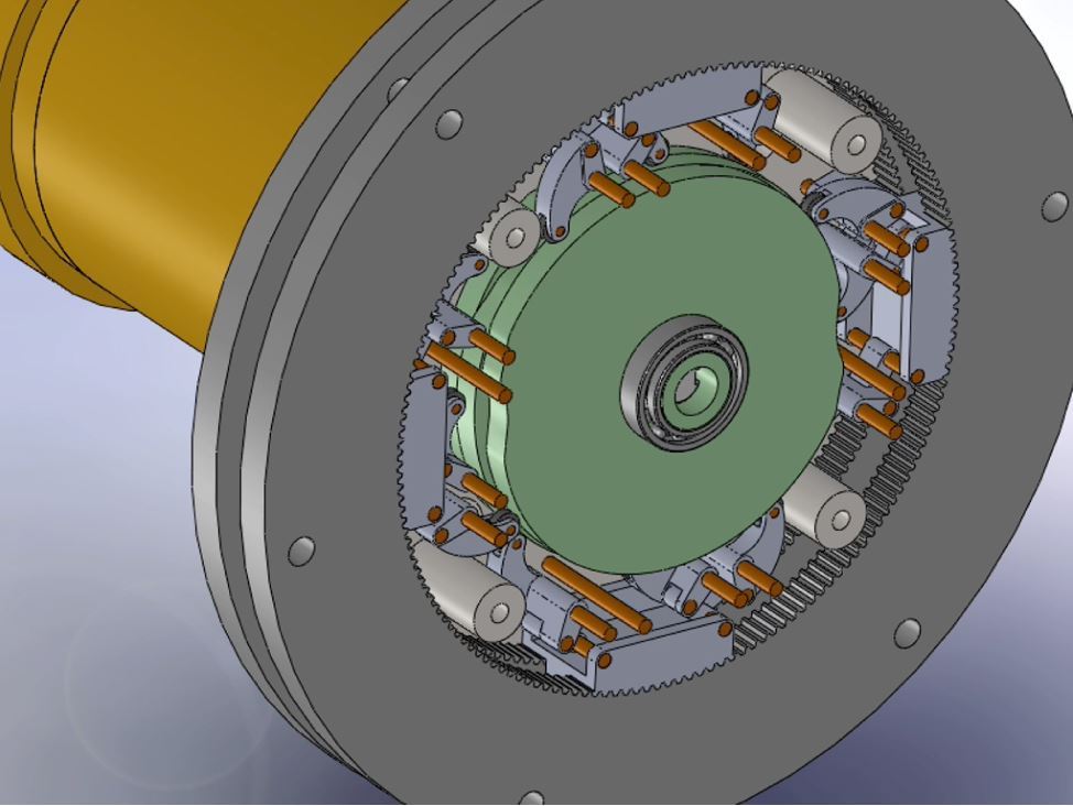
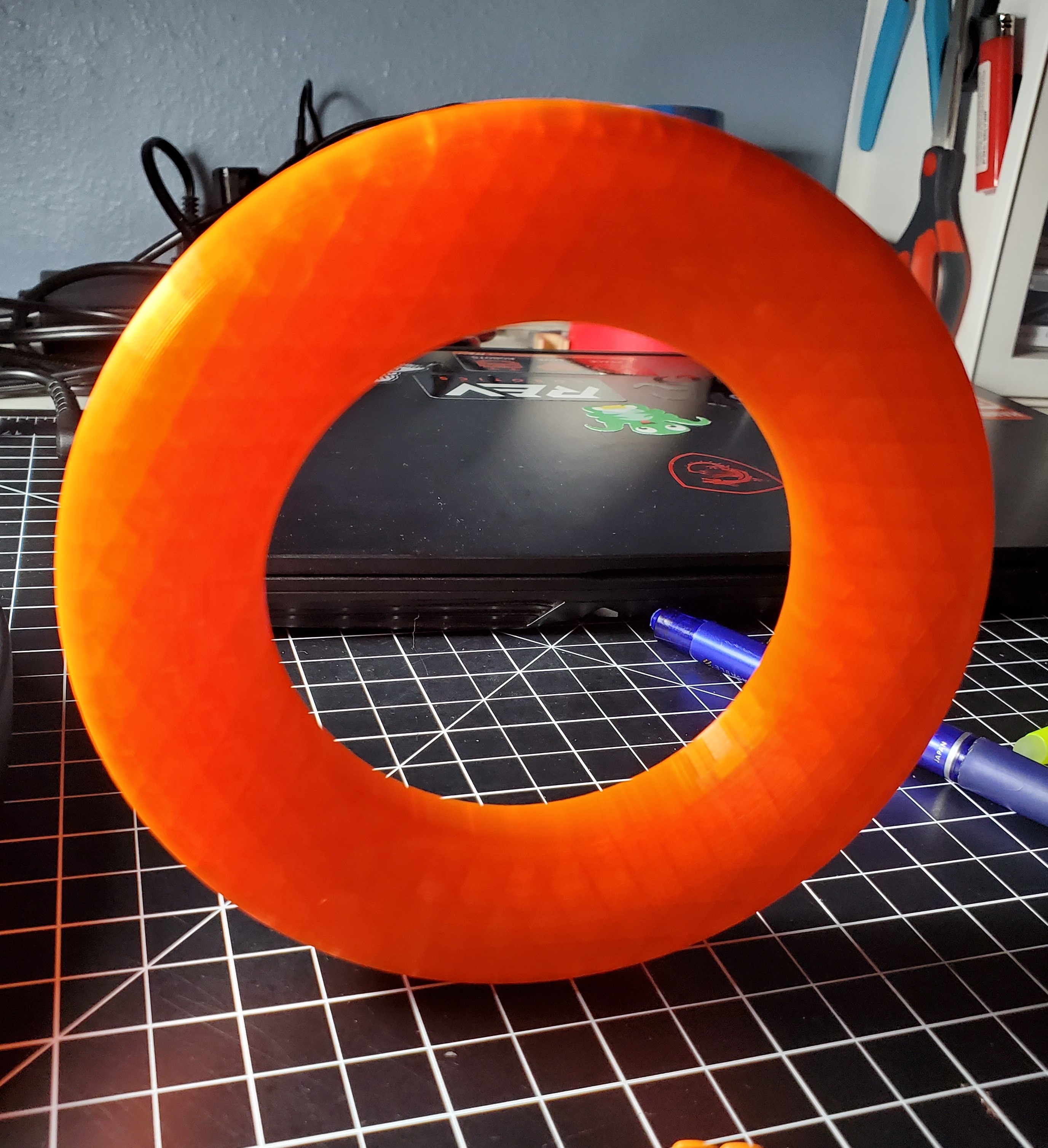
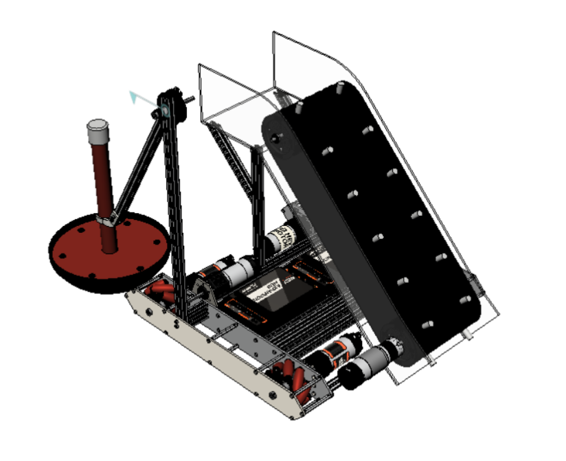
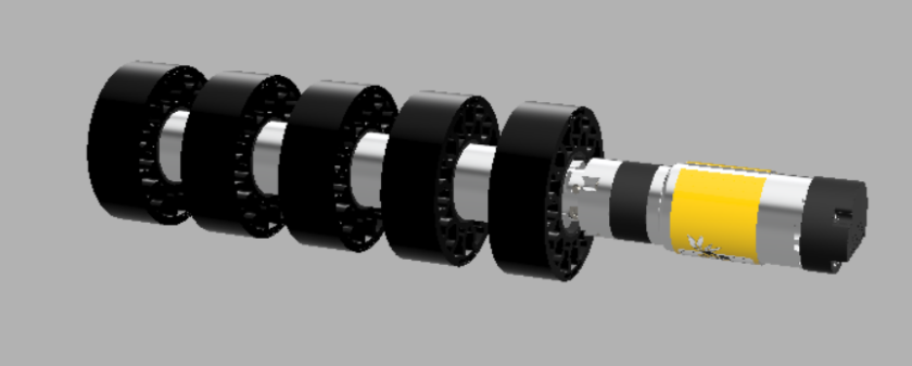
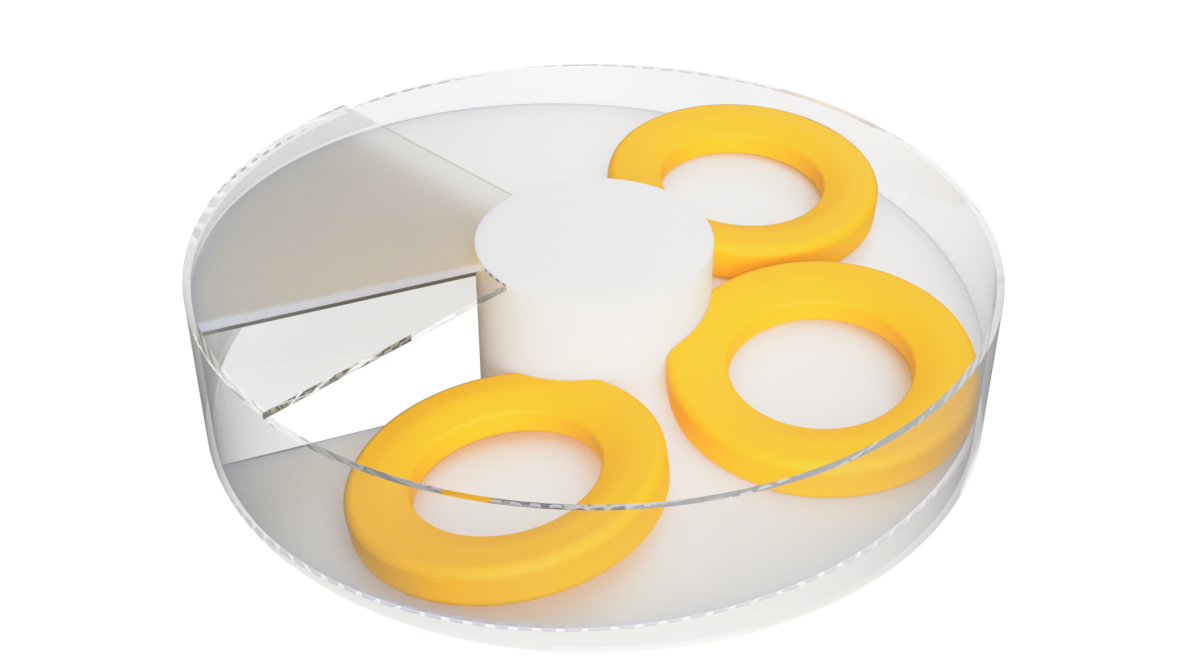
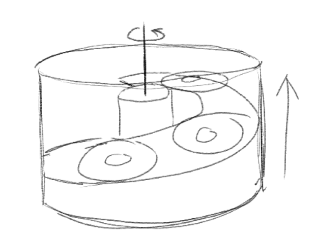
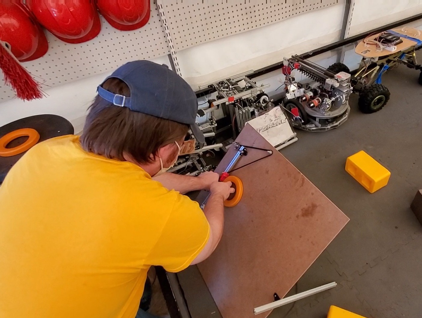
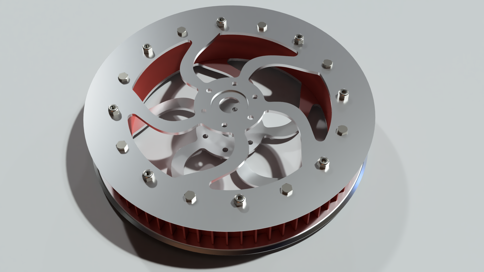
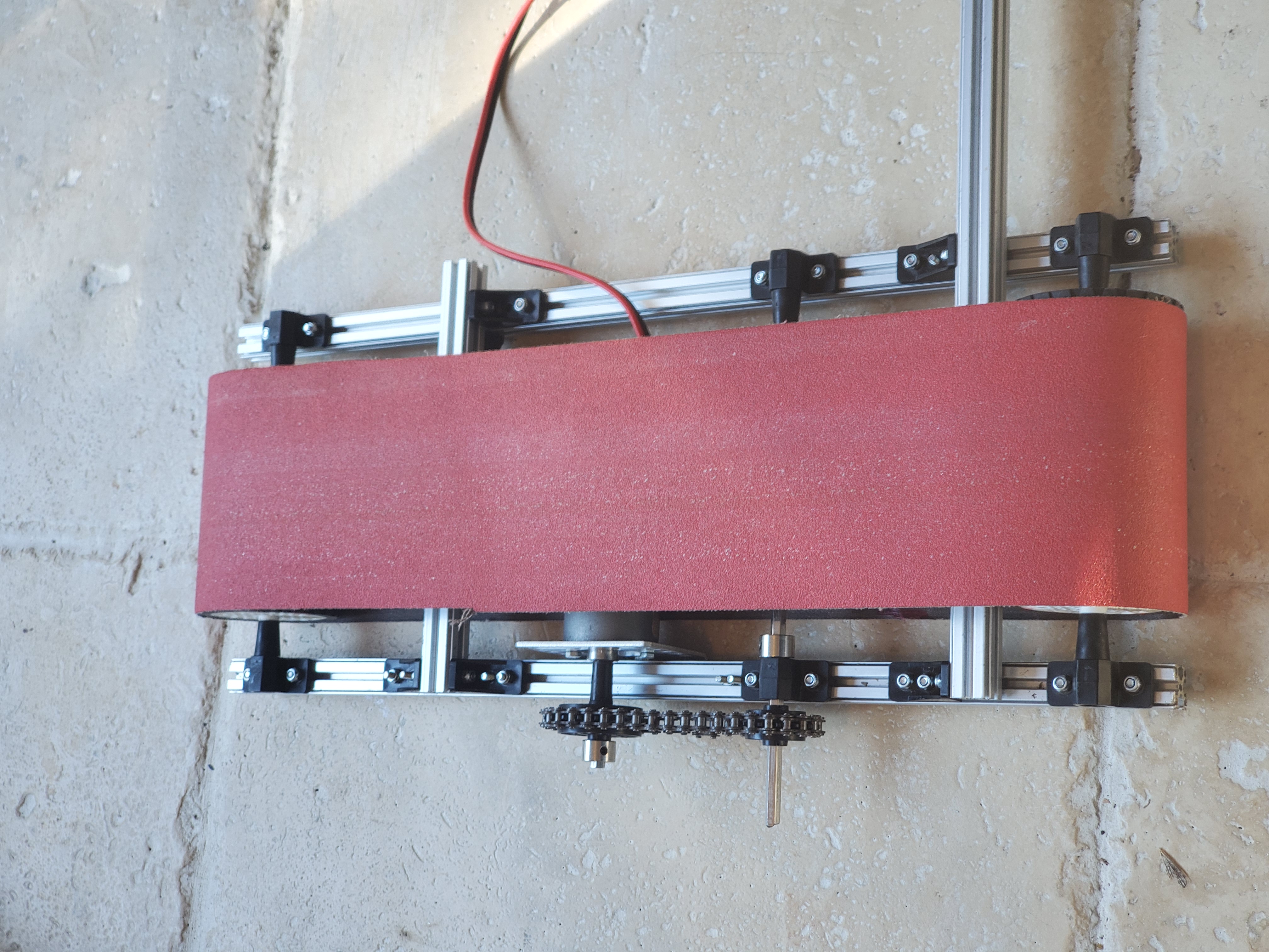
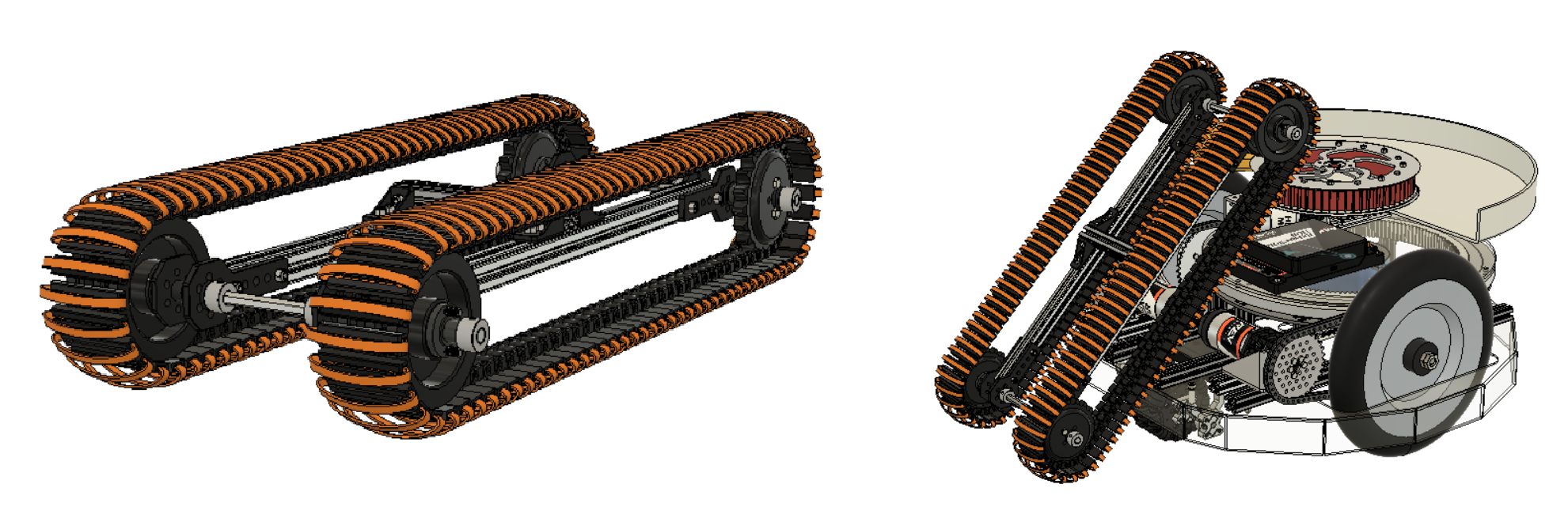
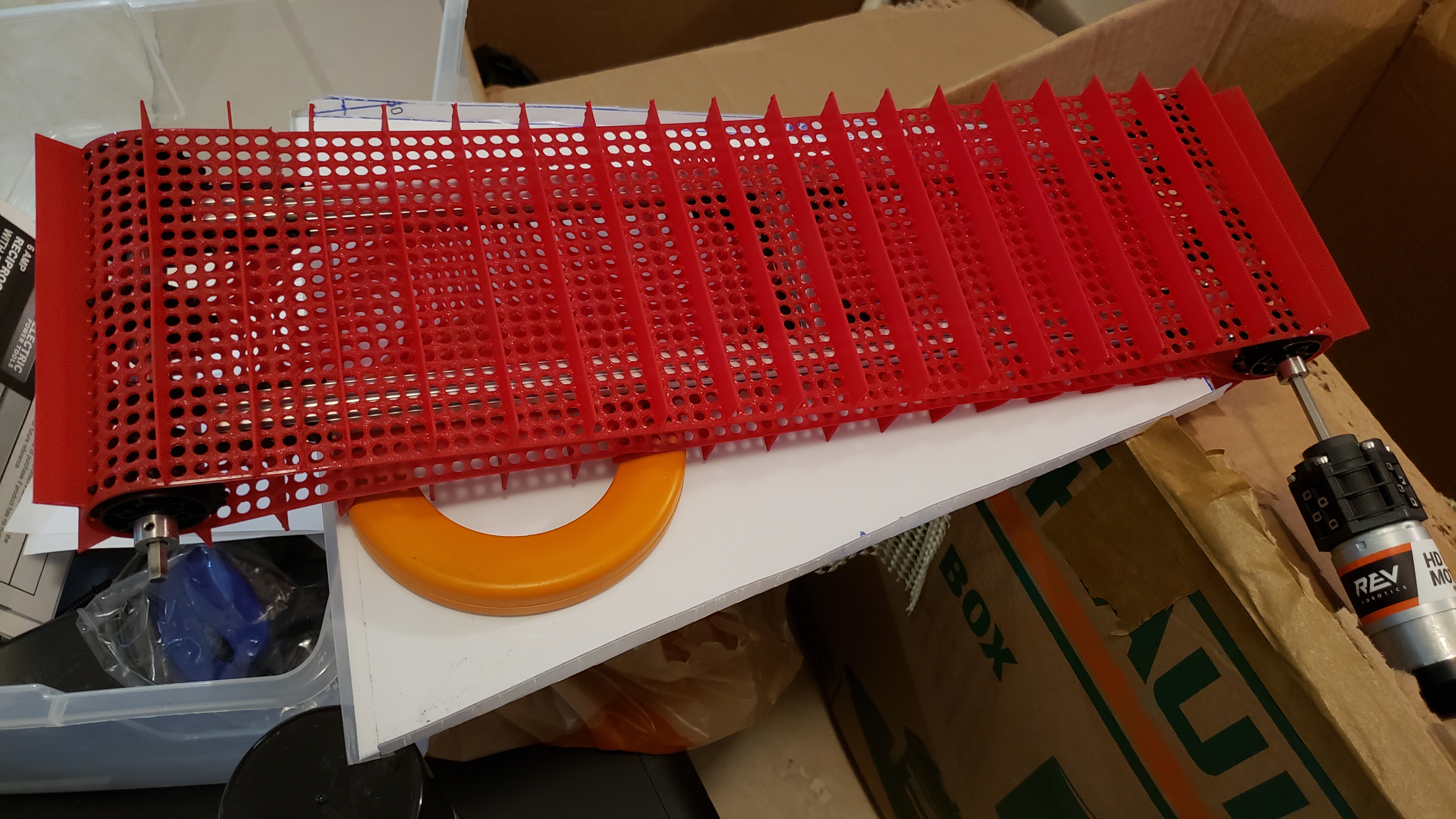
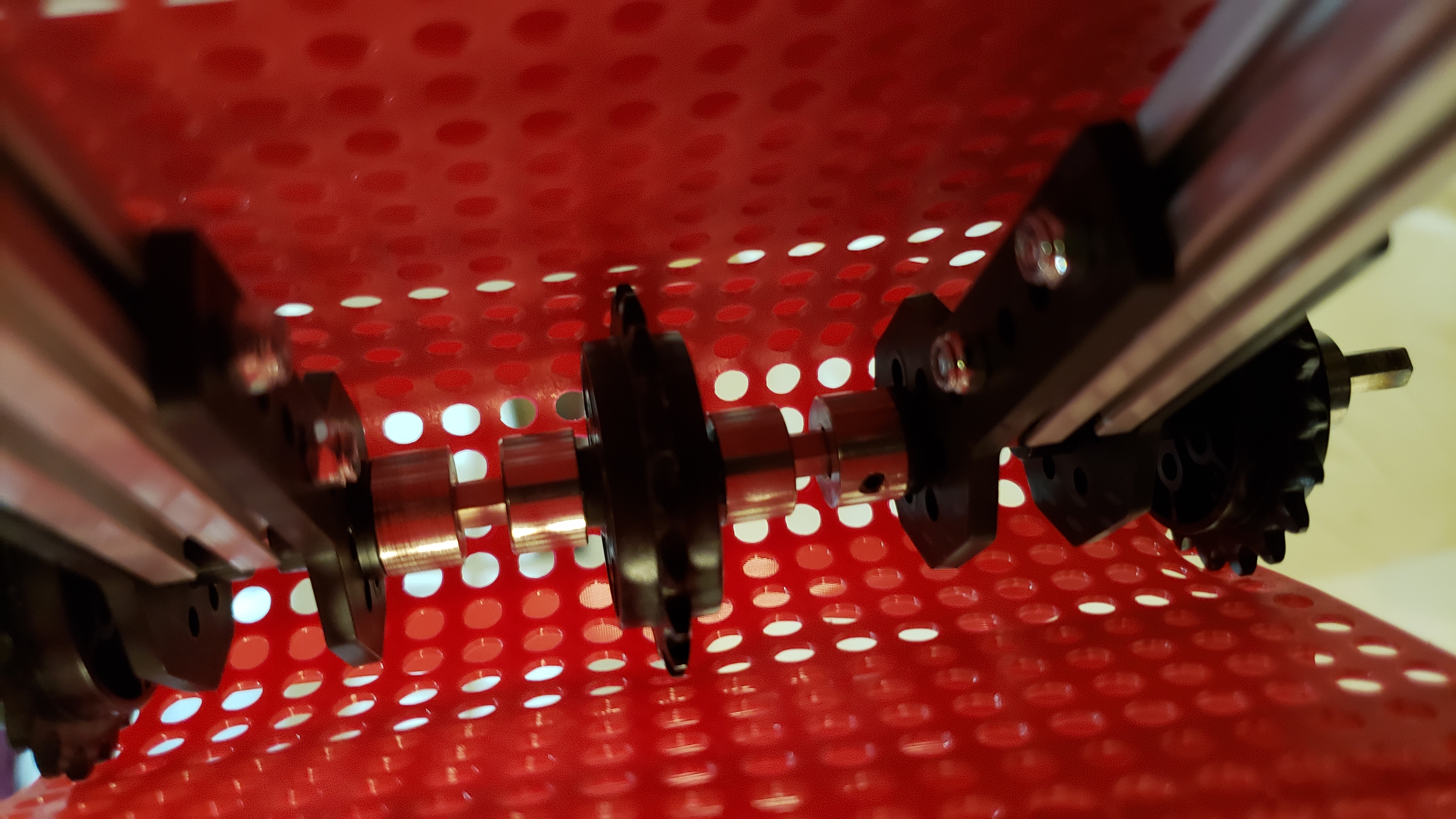
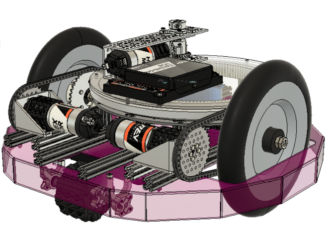
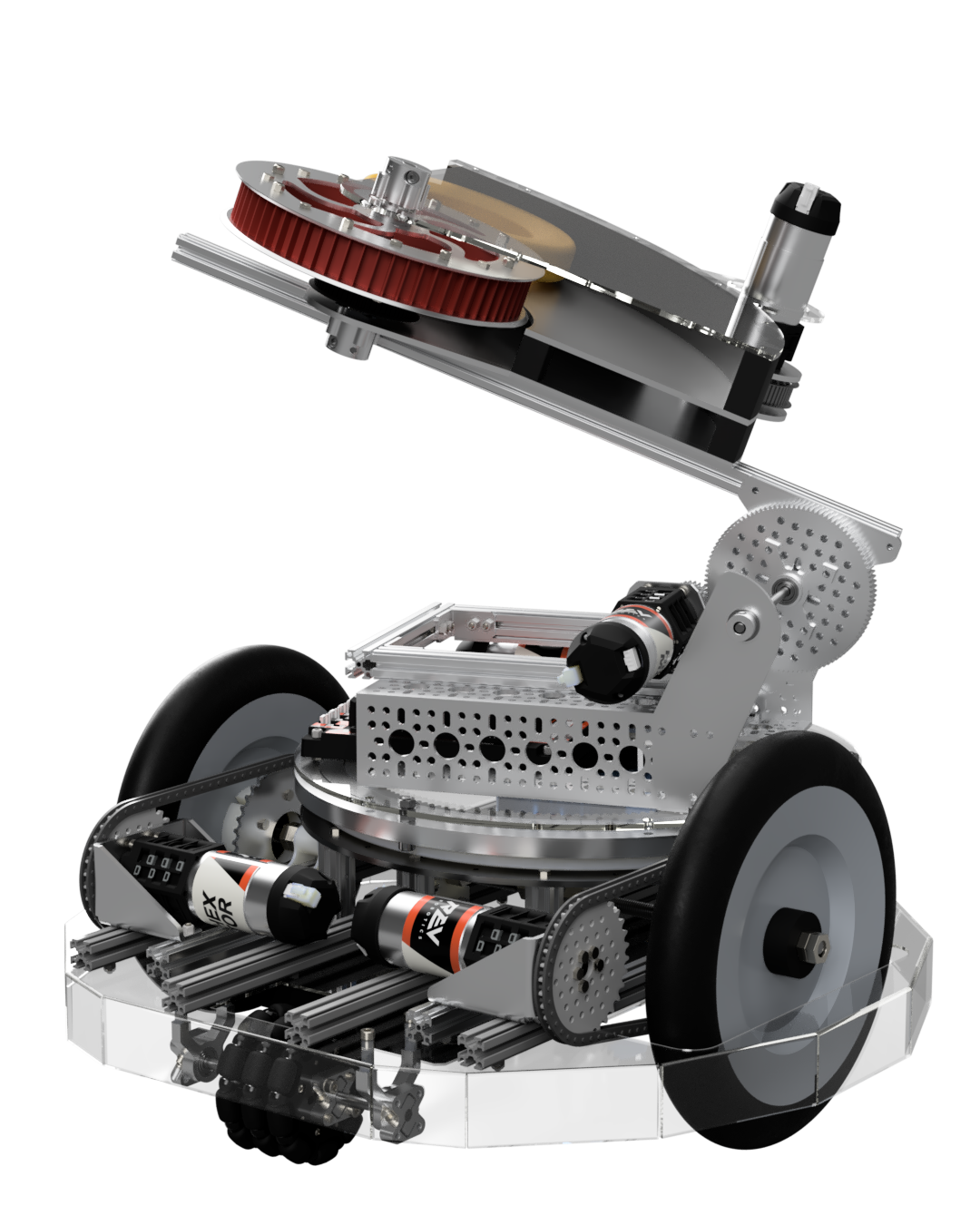
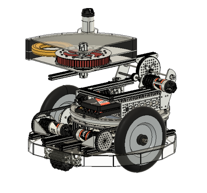
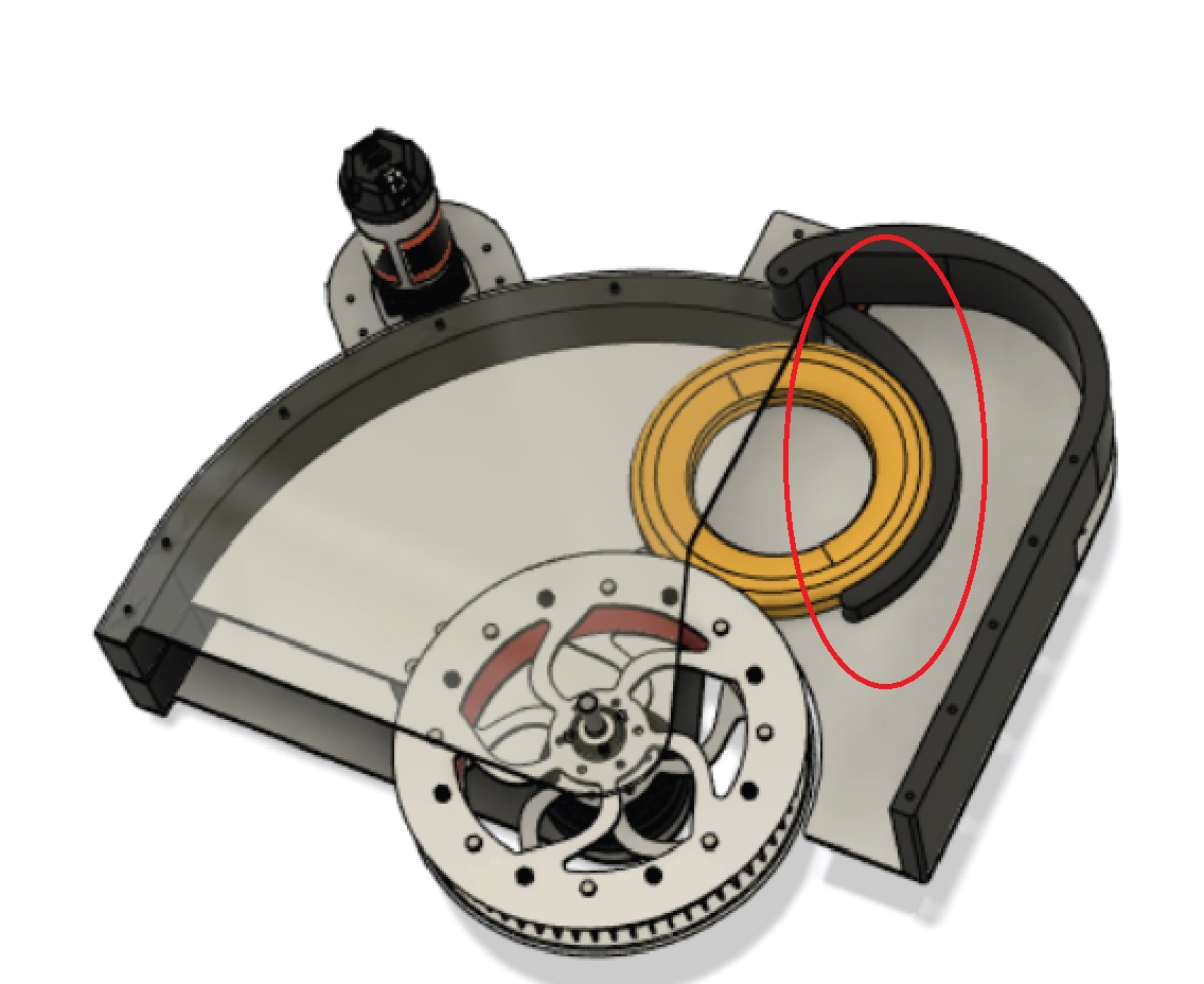
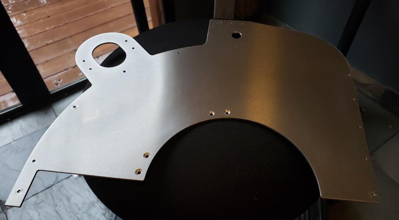
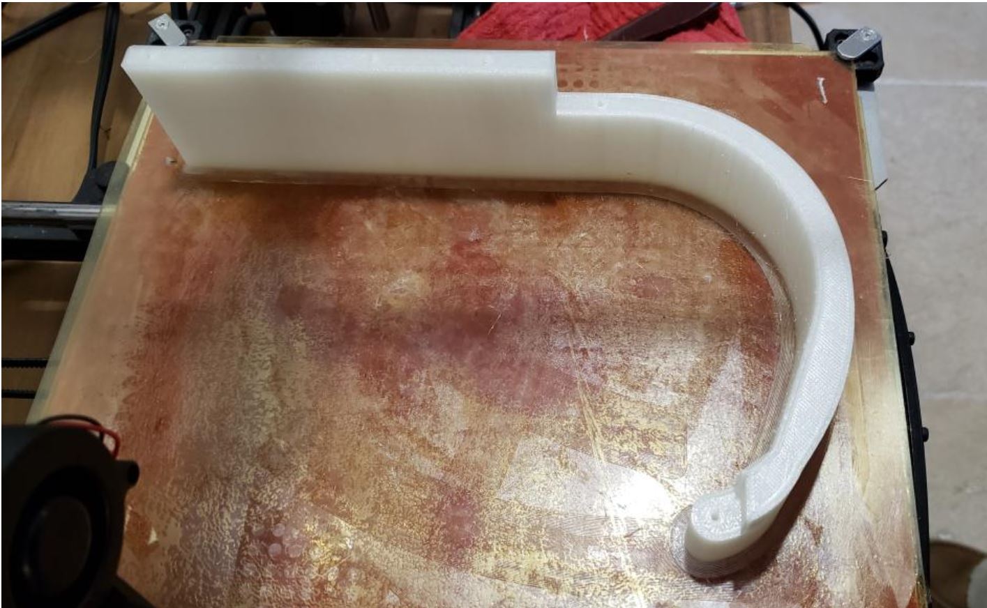
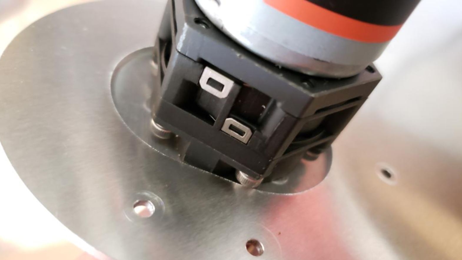
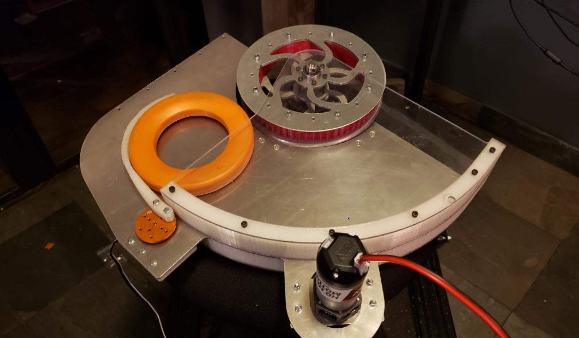
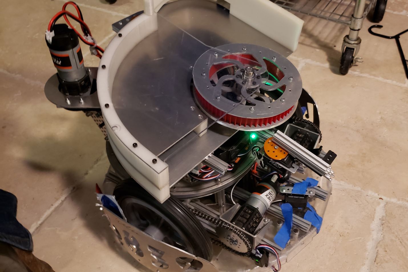
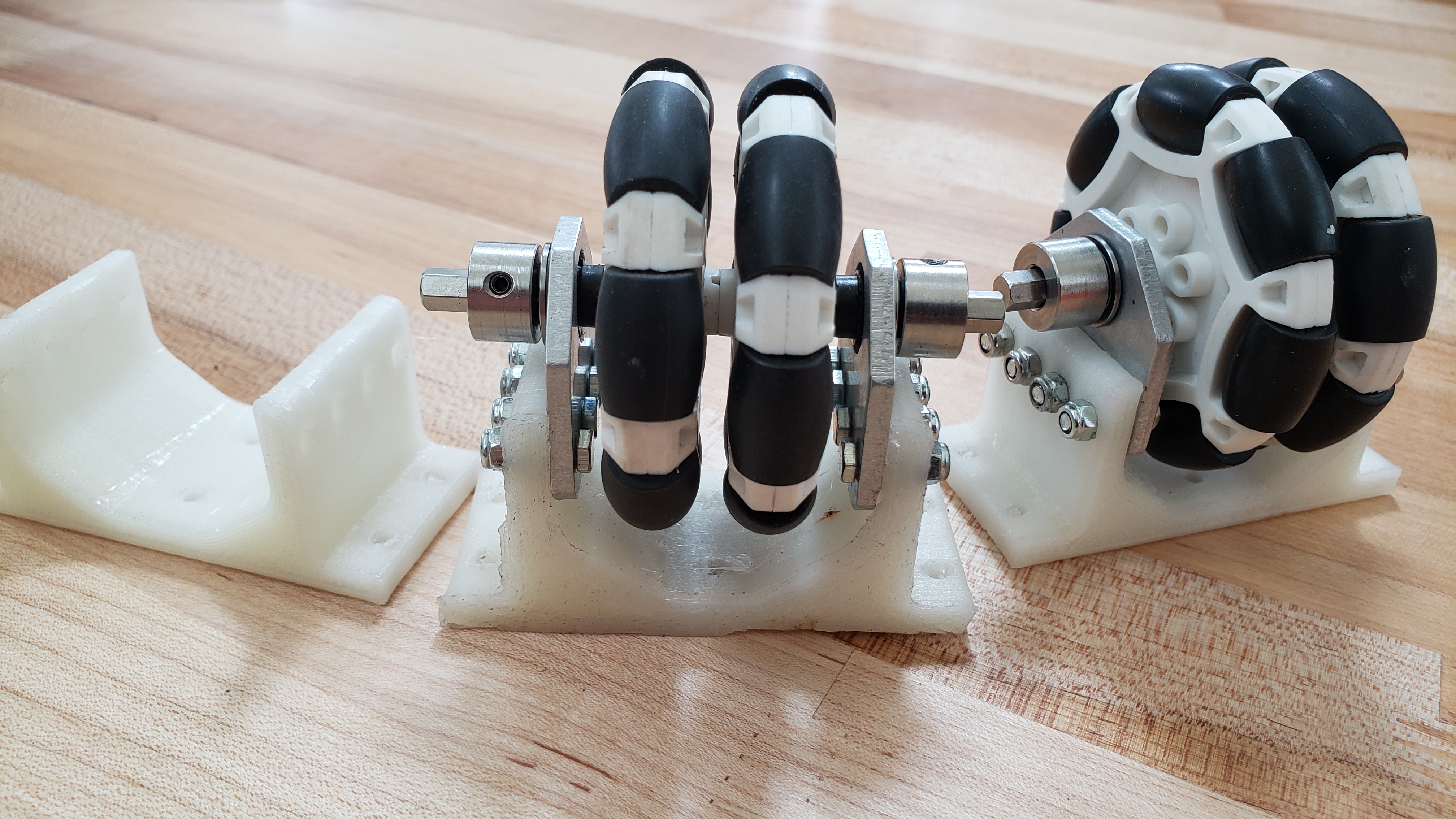
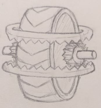
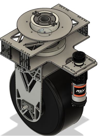
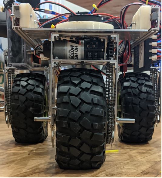
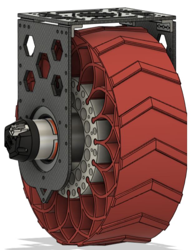
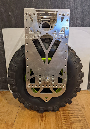
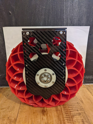
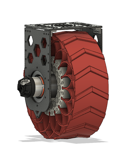
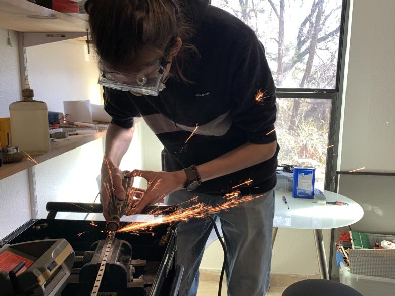
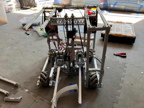
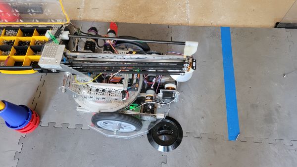
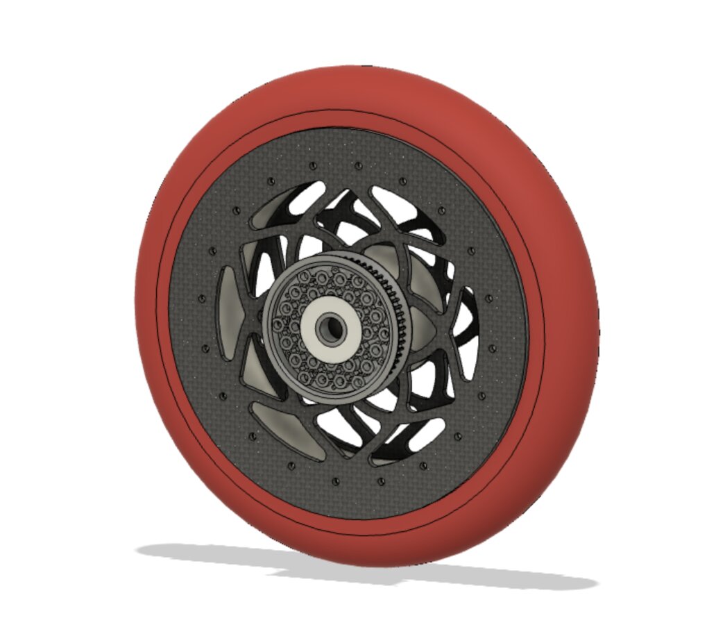
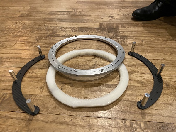
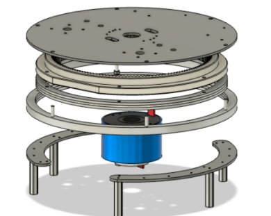
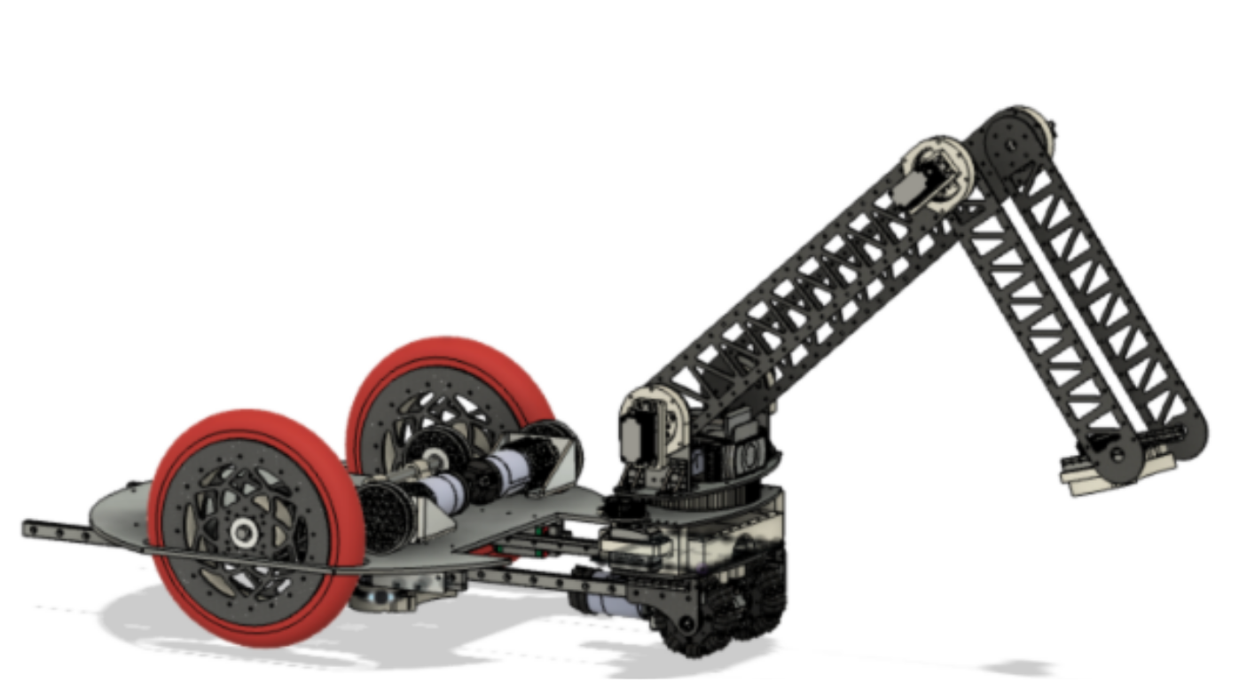
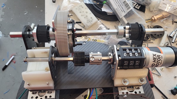
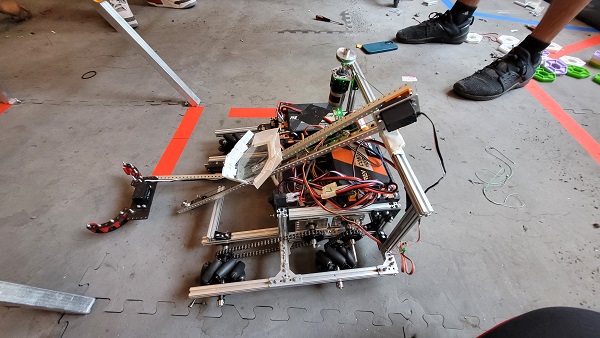
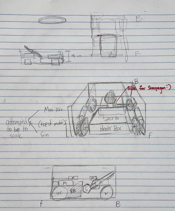
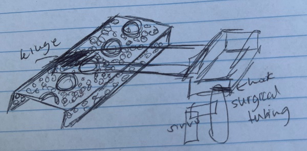
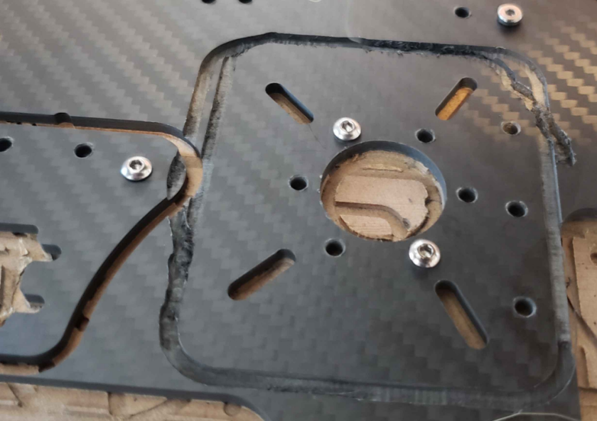
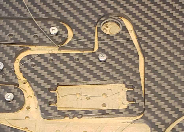
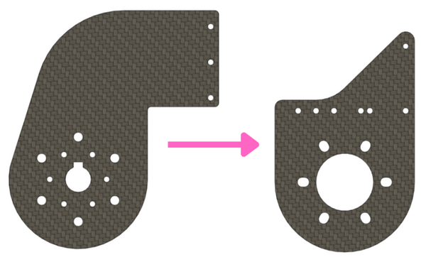
We did this by redesigning our wheel modules and moving the motor further down. Our redesigned wheel modules utilize custom printed "barrier beaters" instead of the rock climbers we used before. These wheels were printed out of ninja flex and nylon and utilized a Gothic Arch design inspired by Monash University's rover wheels. The custom wheel modules used custom carbon-fiber plates and holes in the nylon hub to help reduce weight. Overall, these wheels were excellent at traversing the barriers, weighed less, and the wheel module allowed the motor to drop 5 inches in height. This led to a lower center of mass for the robot.
You can see from these free-body diagrams that as we lower the vertical component of the normal force, the overall rotational torque exerted by the swerve module is decreased, which inspired our decisions to lower the center of mass.
We did this by redesigning our wheel modules and moving the motor further down. Our redesigned wheel modules utilize custom printed "barrier beaters" instead of the rock climbers we used before. These wheels were printed out of ninja flex and nylon and utilized a Gothic Arch design inspired by Monash University's rover wheels. The custom wheel modules used custom carbon-fiber plates and holes in the nylon hub to help reduce weight. Overall, these wheels were excellent at traversing the barriers, weighed less, and the wheel module allowed the motor to drop 5 inches in height. This led to a lower center of mass for the robot.
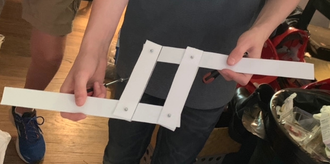
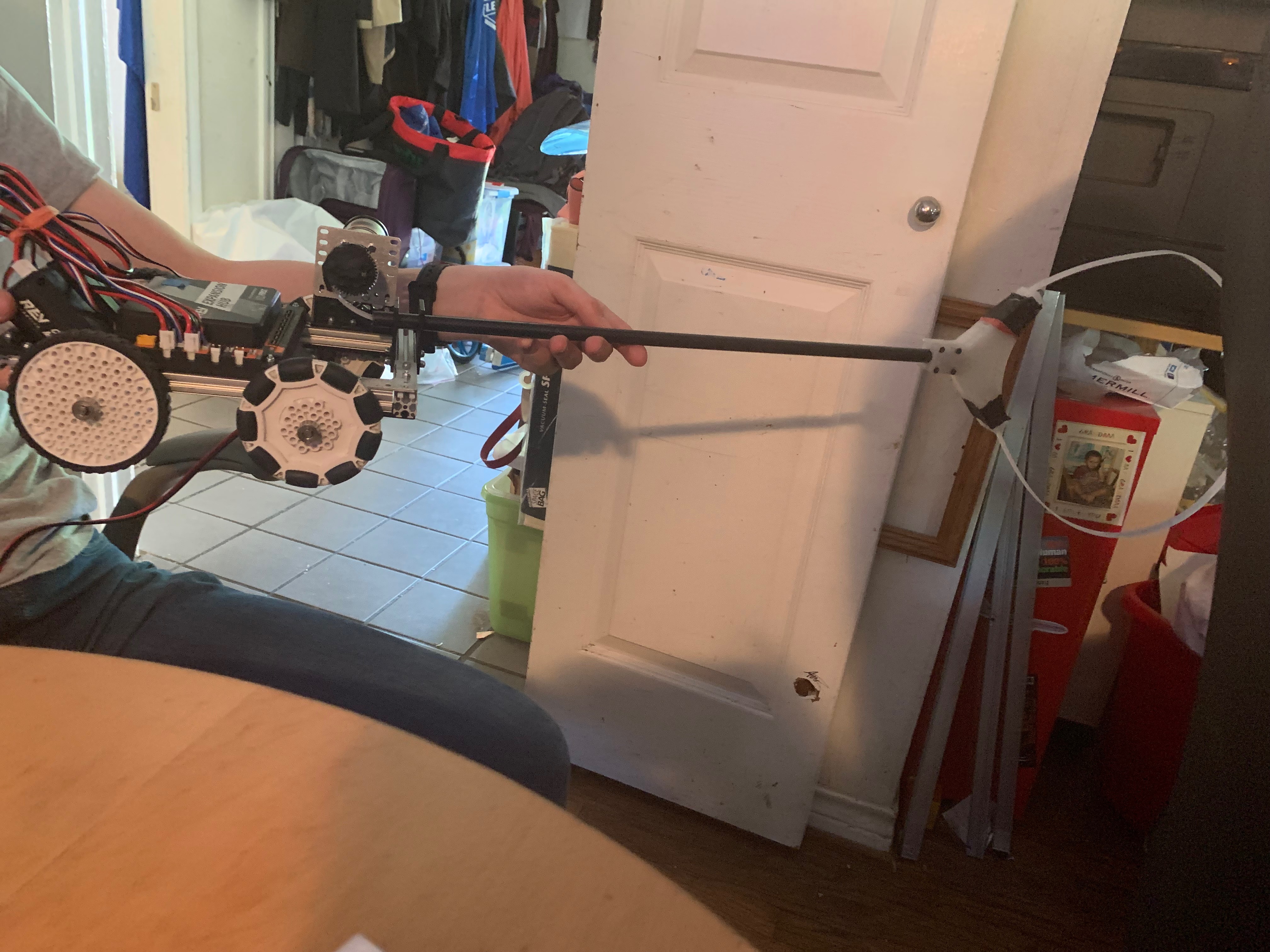
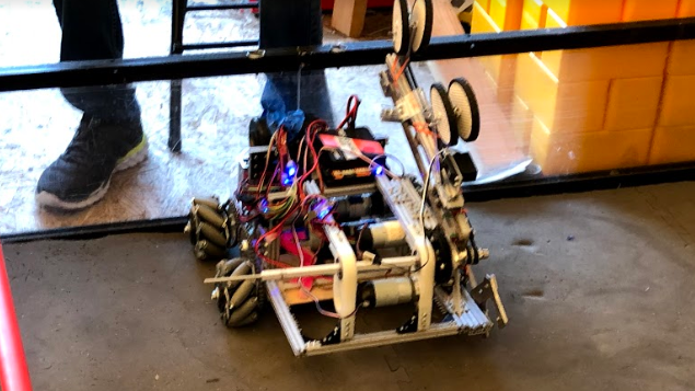
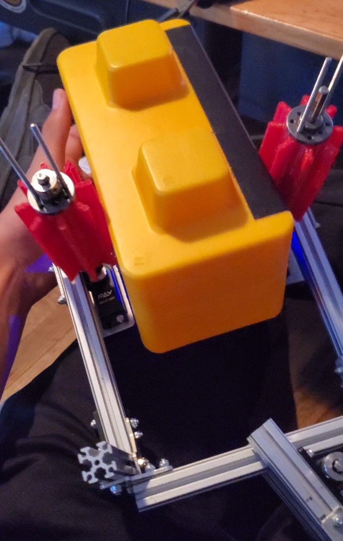
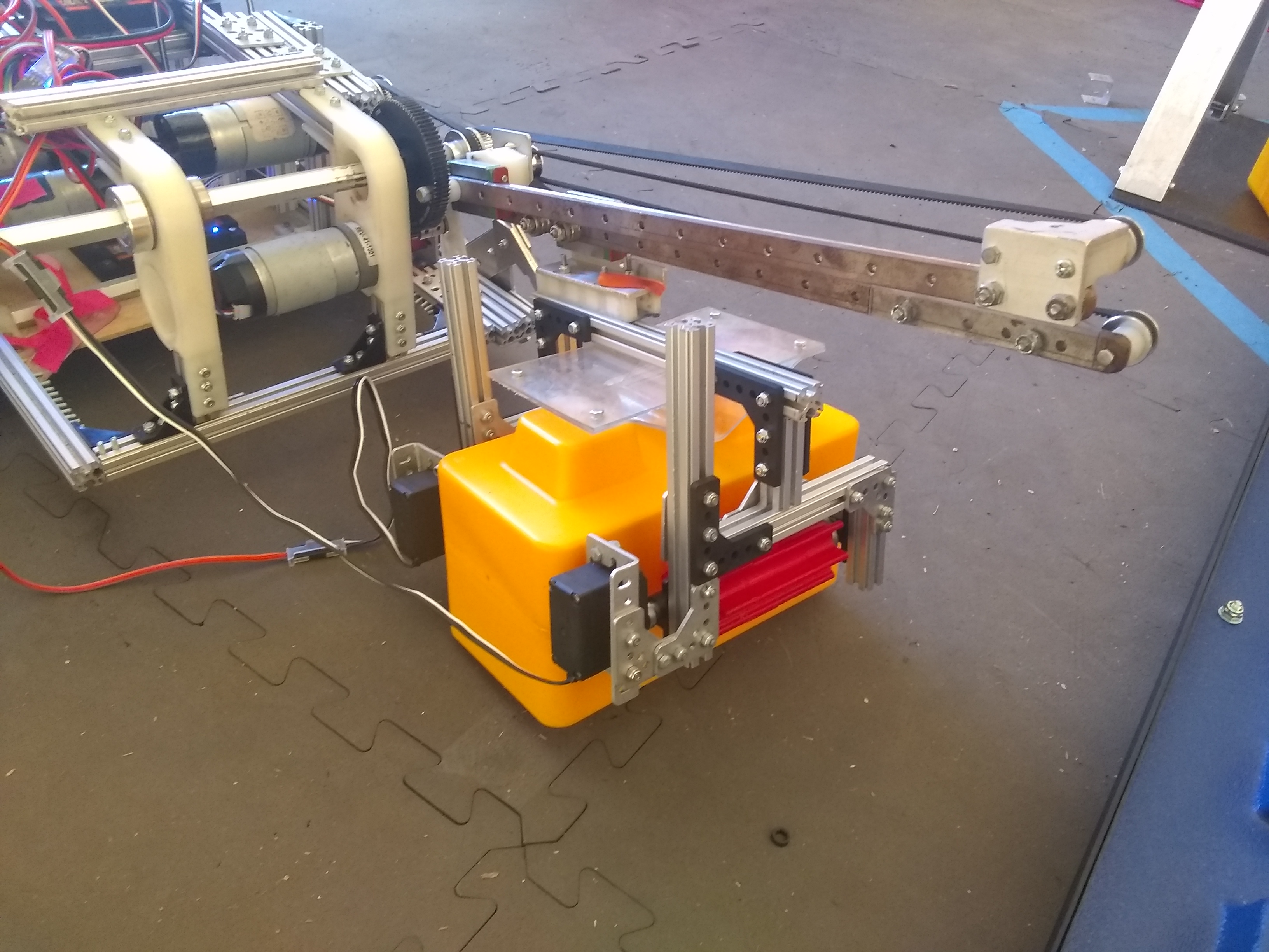
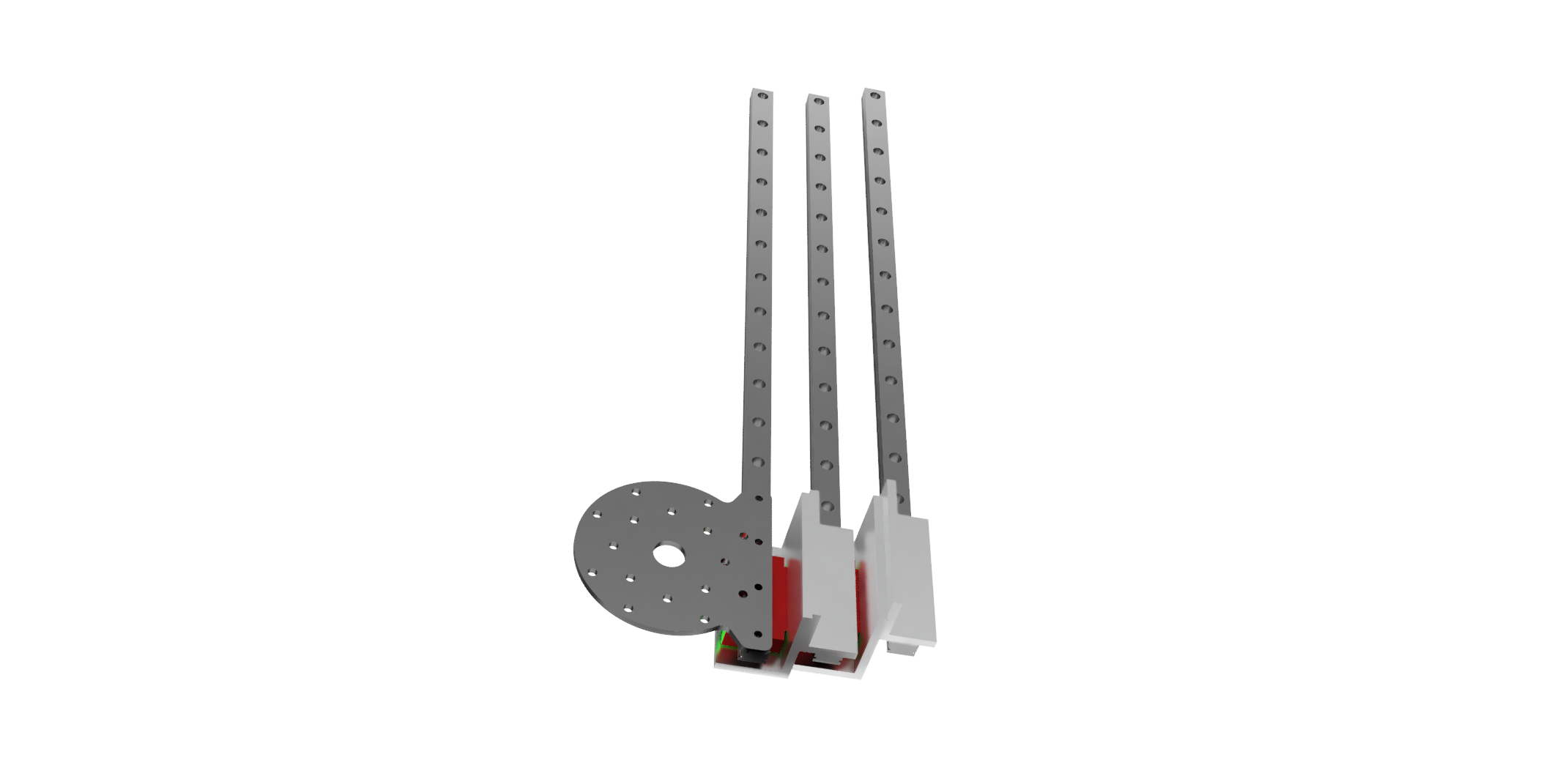
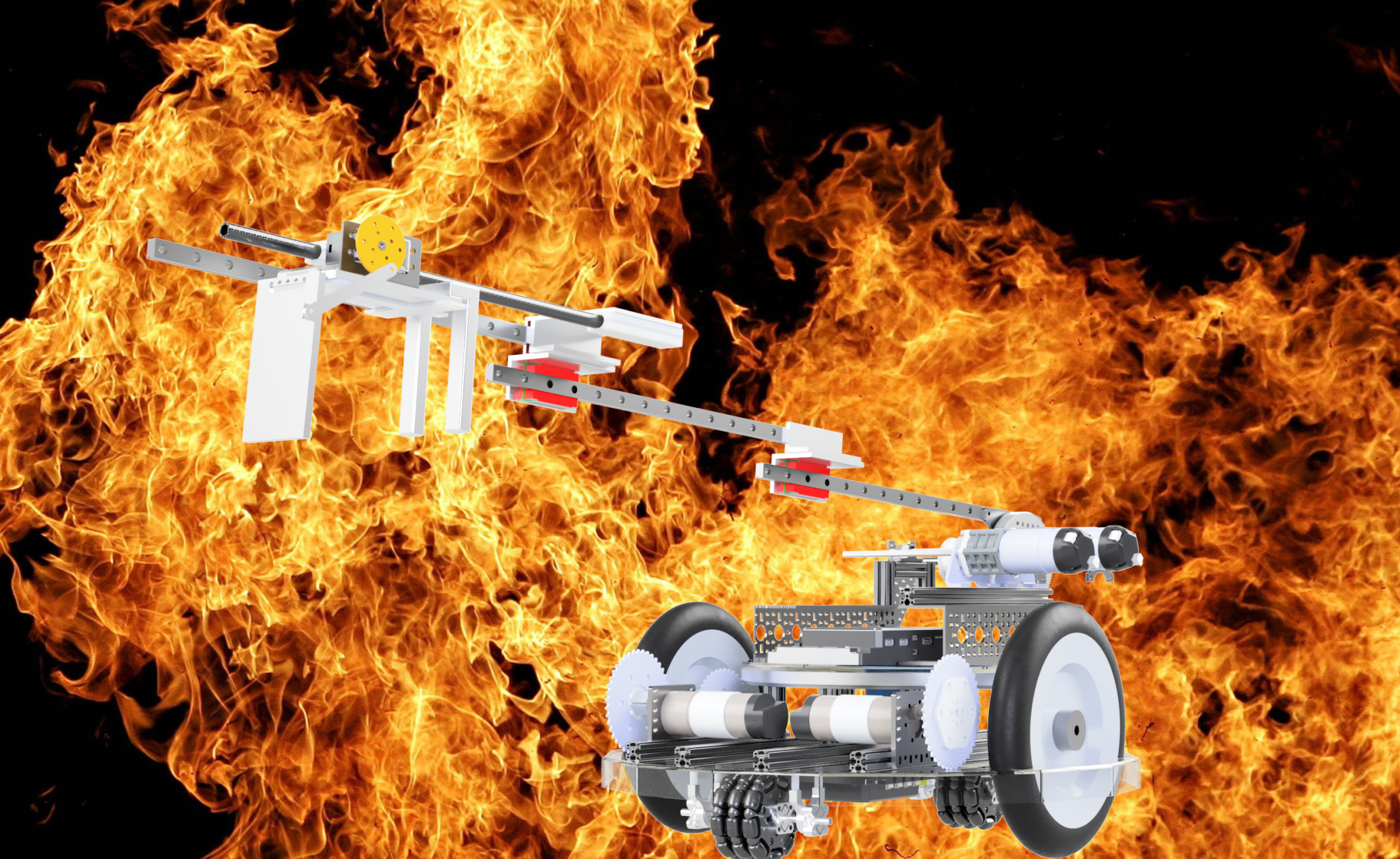
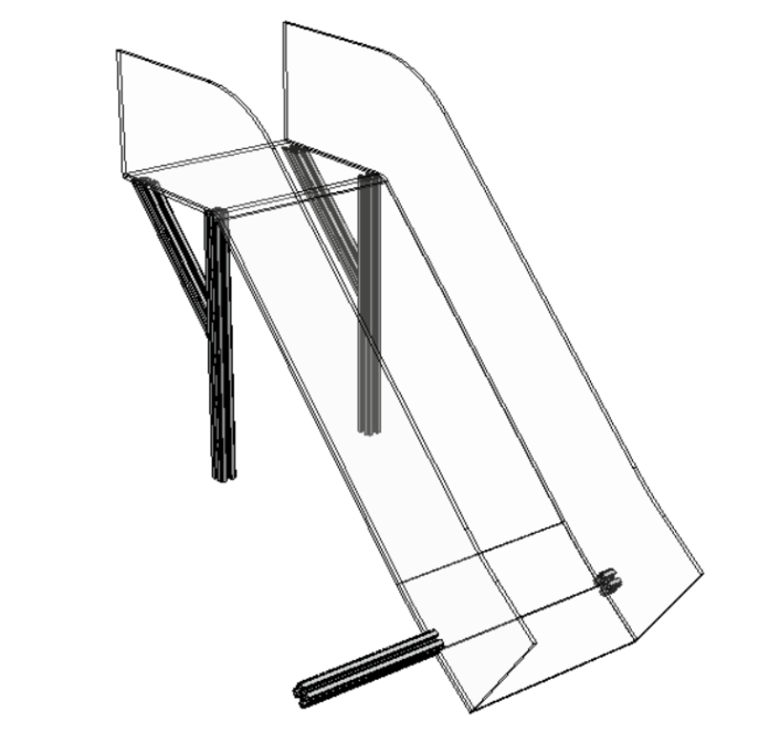
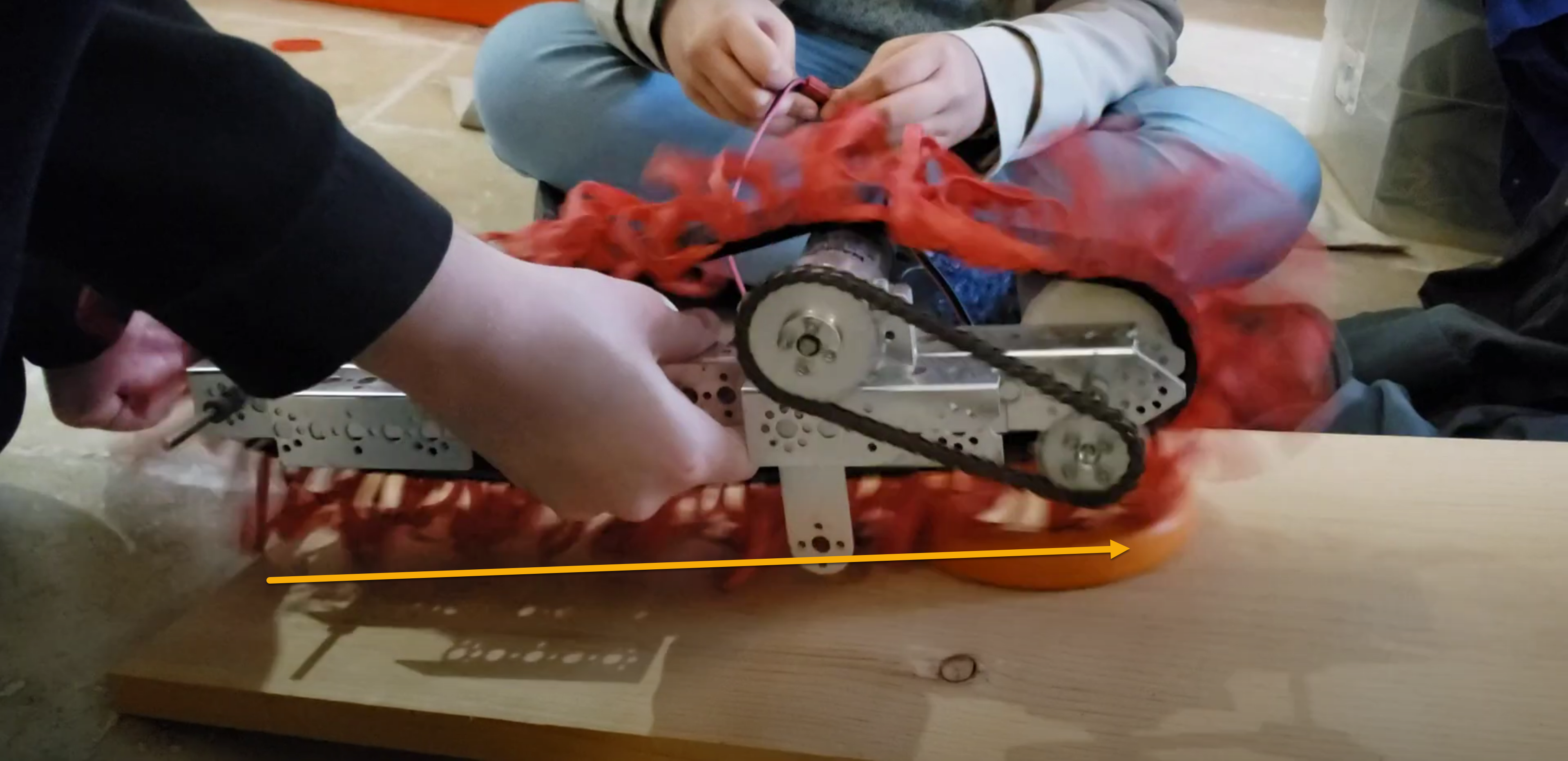
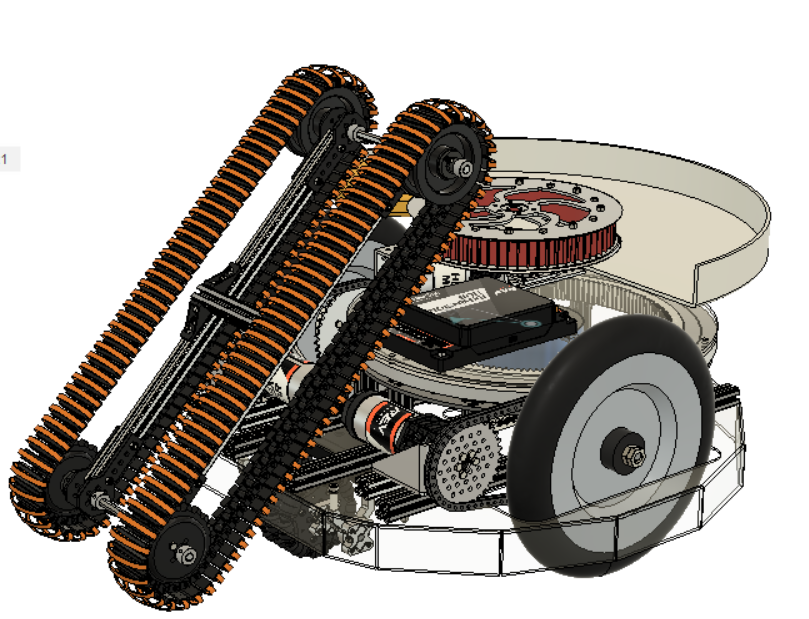
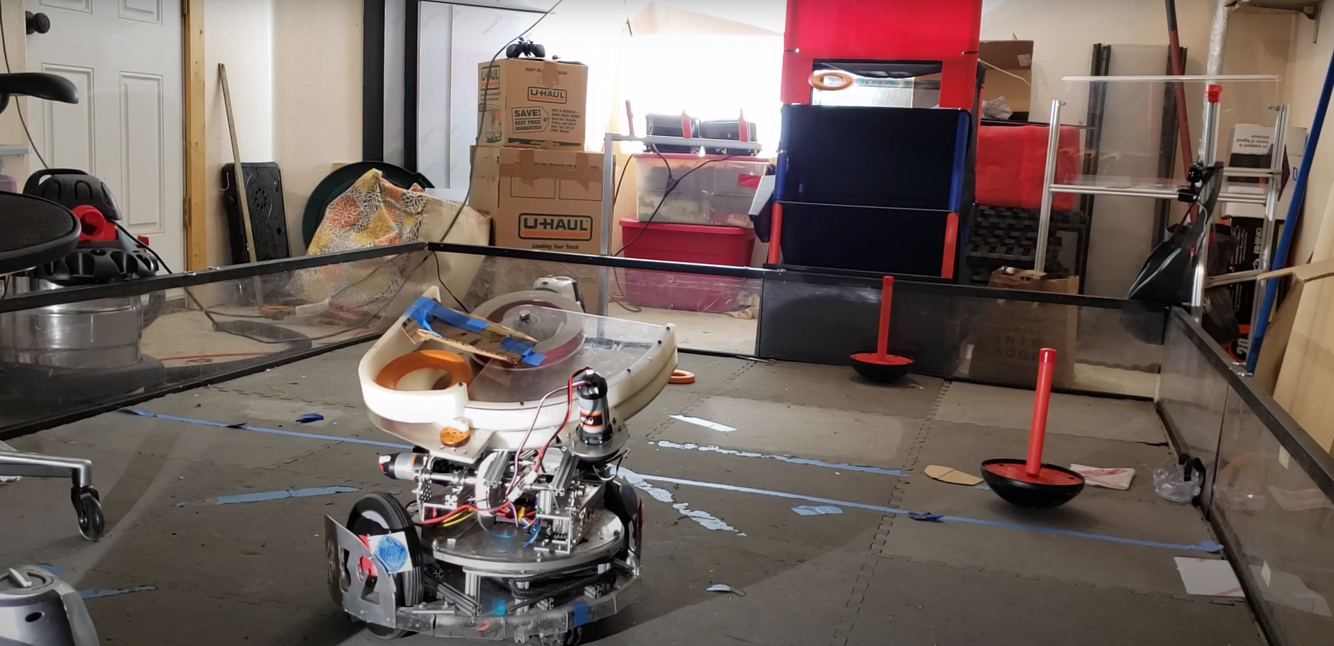
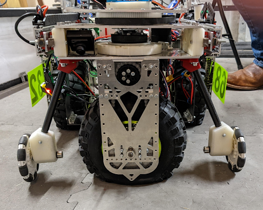
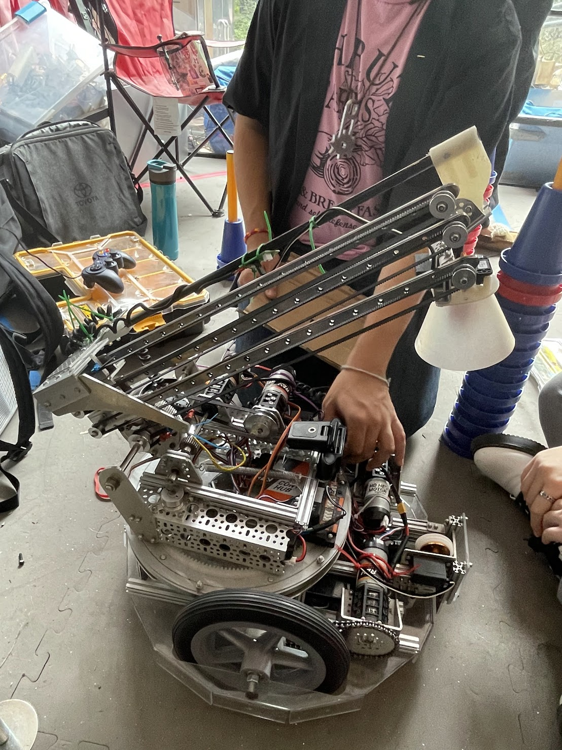
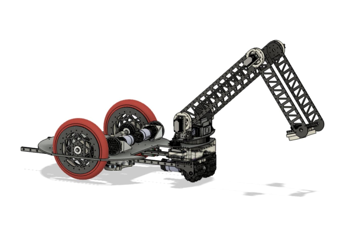
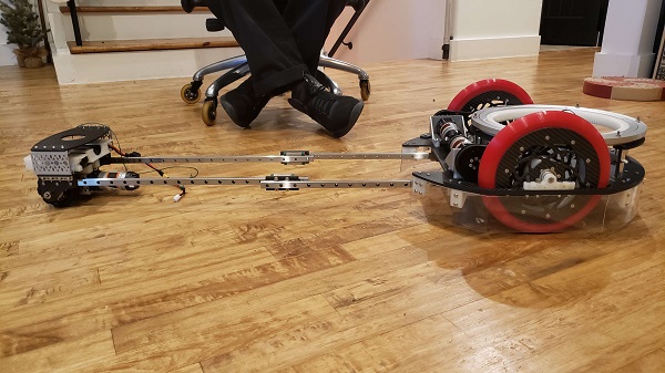
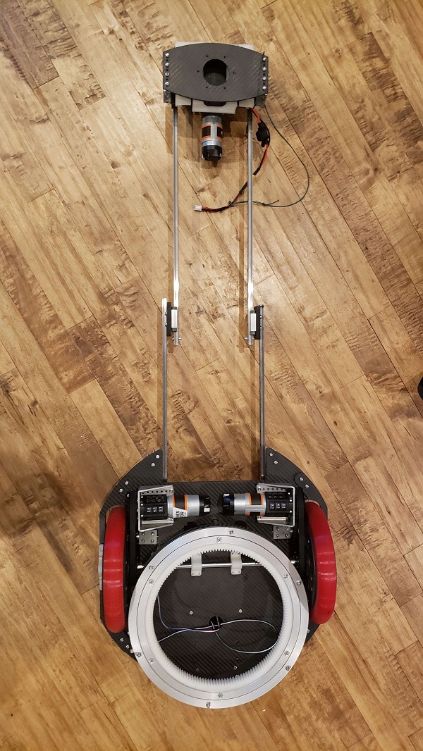
 However, in the situation that the crane and robot extension did lead to the center of mass nearing the base, we installed an outrigger system as a preventative measure. An outrigger is essentially a beam that extends from a robot that is used to improve stability. Our outriggers used omni wheels and functioned similarly to training wheels, preventing the robot from tipping over when the crane moves out and extends.
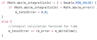
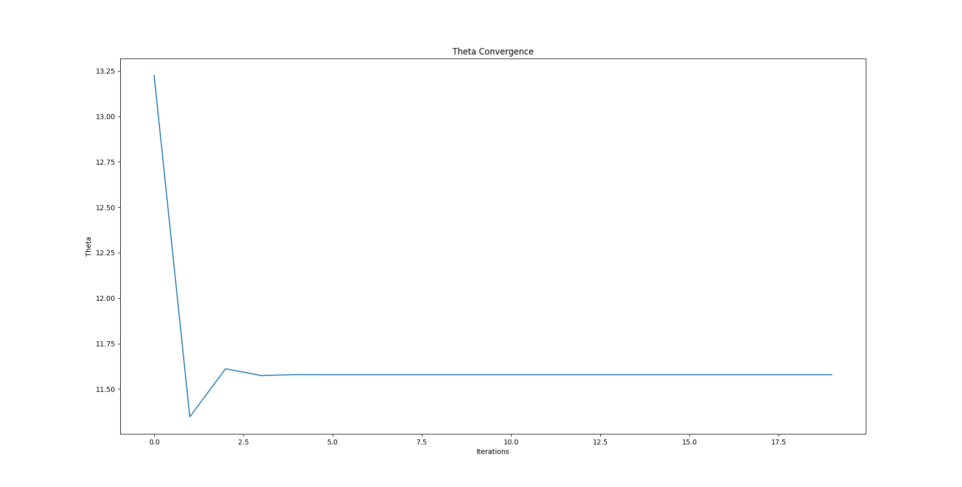
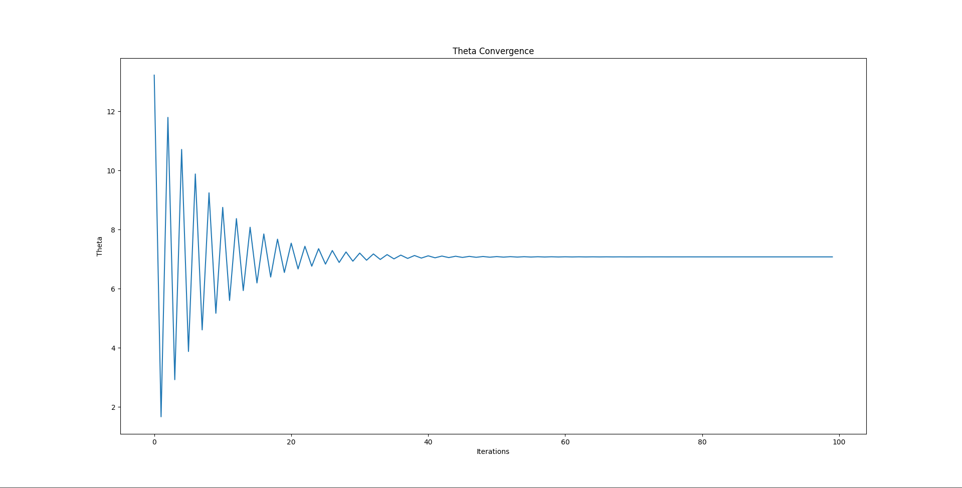
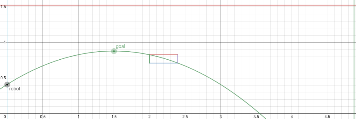
 Finally, we implemented some code changes to help deal with this problem, building anti-tipping limiters which allowed for gradual acceleration. This prevented the sudden acceleration mentioned earlier which was a cause of our tipping issue. We also programmed in pre-set arm locations to help keep the center of mass near the wheelbase, making sure that the center of mass never passes the base of the actual robot.


.jpg)
.jpg)
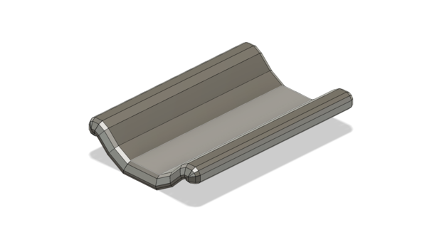

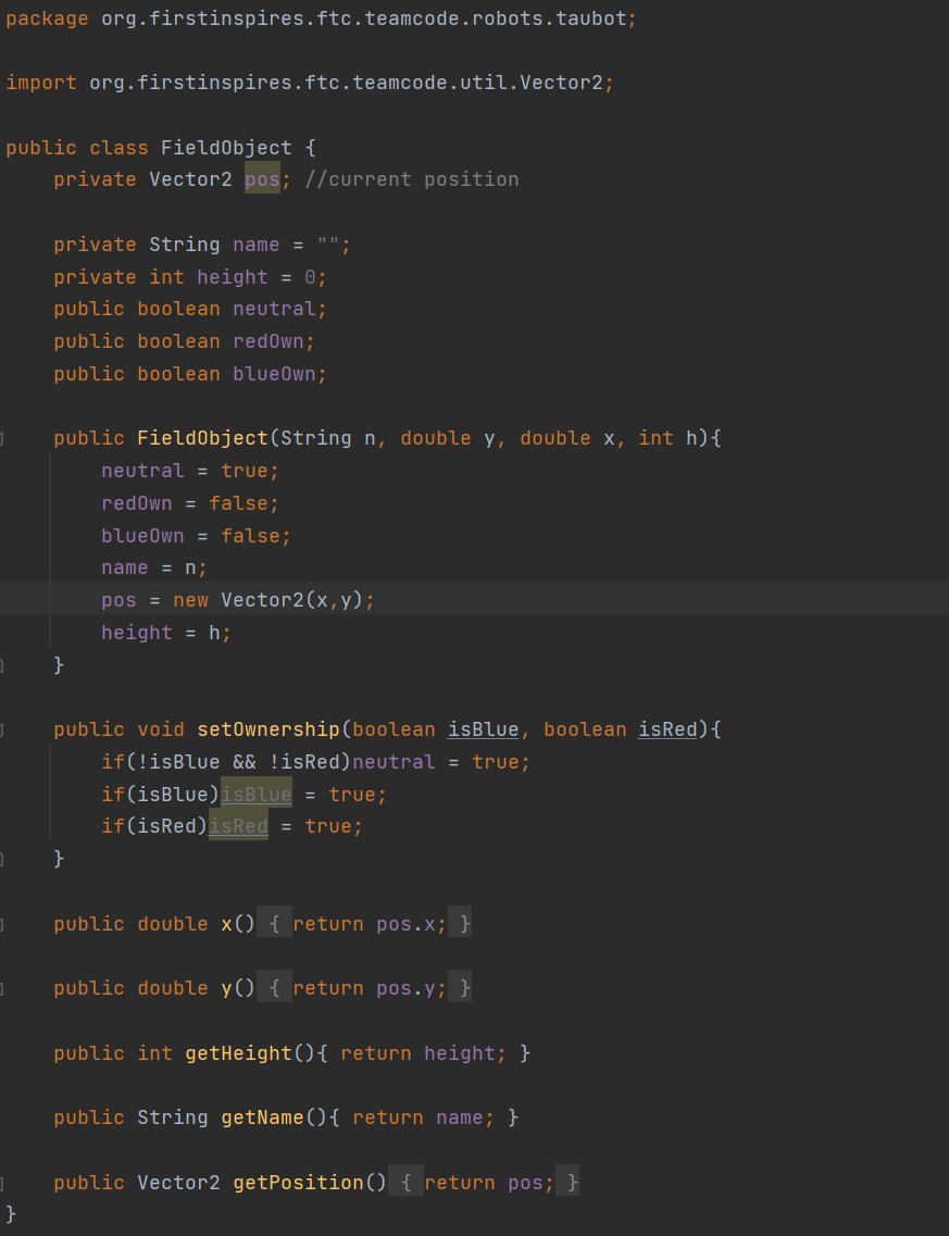
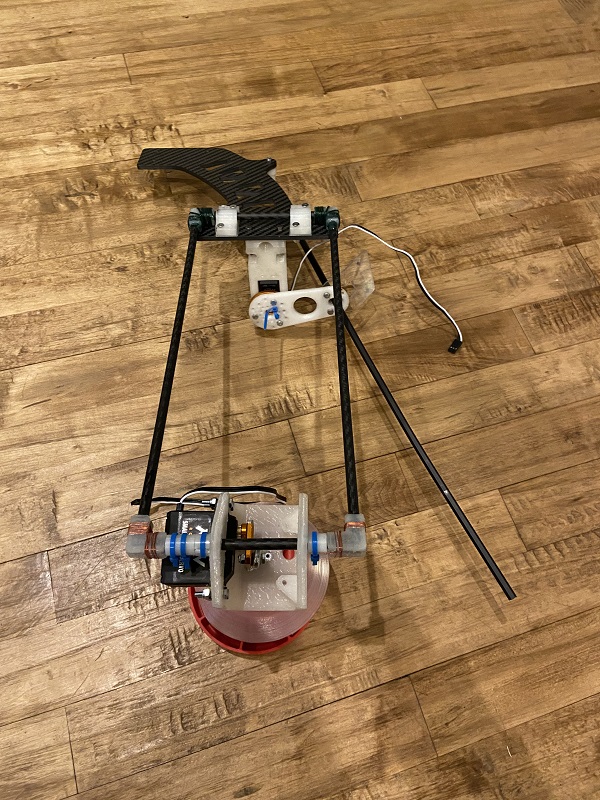
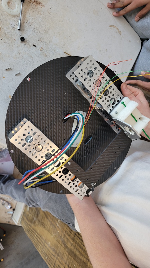
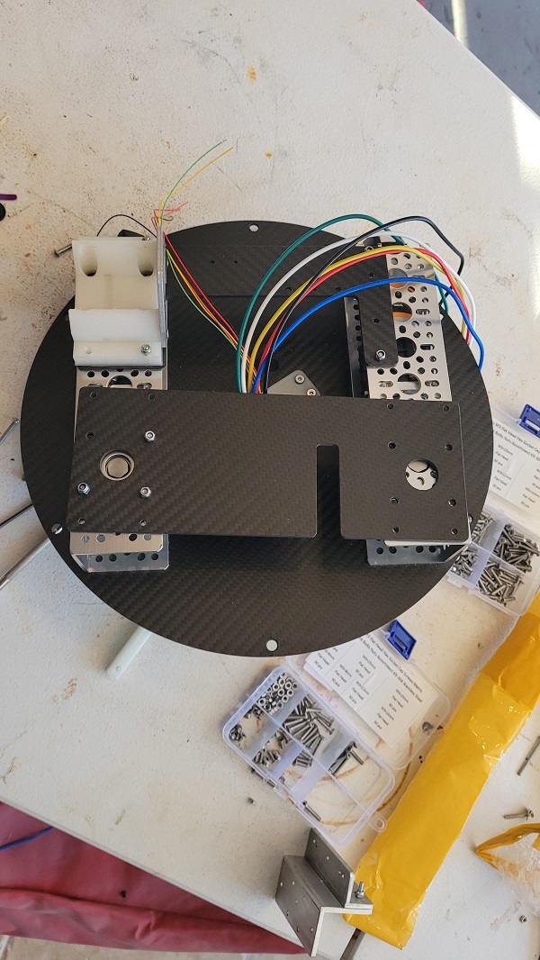

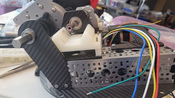
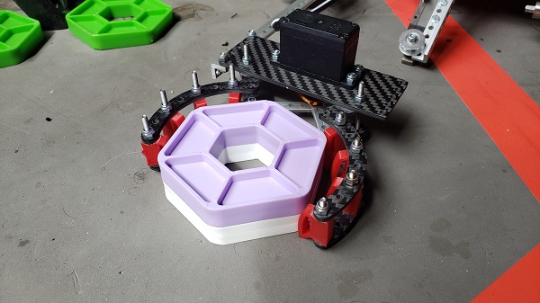
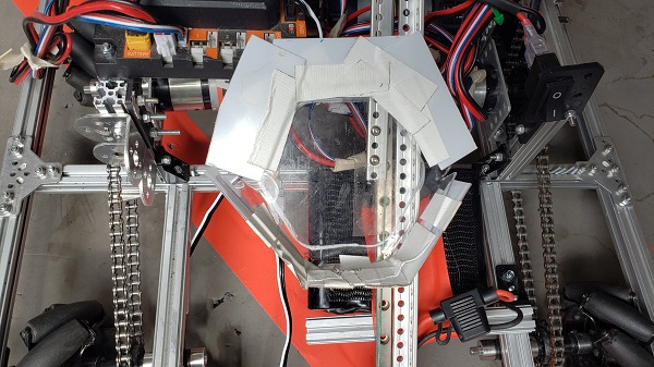
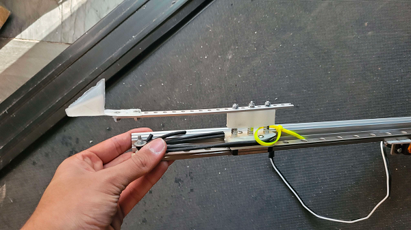
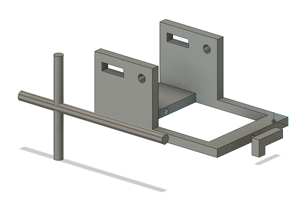

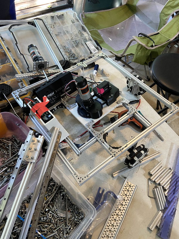
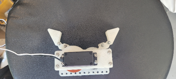
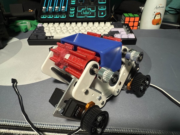
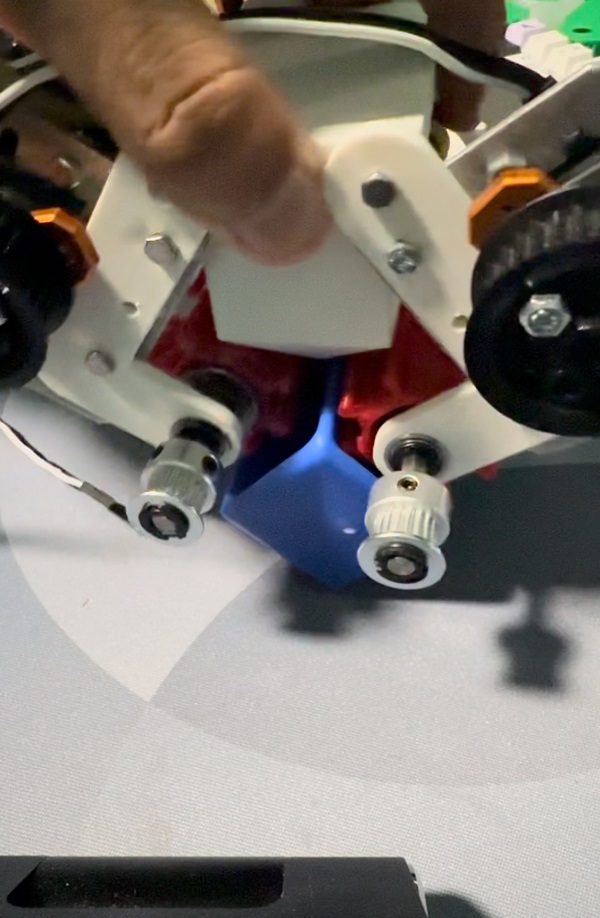
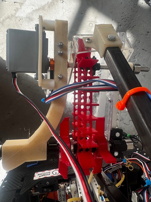
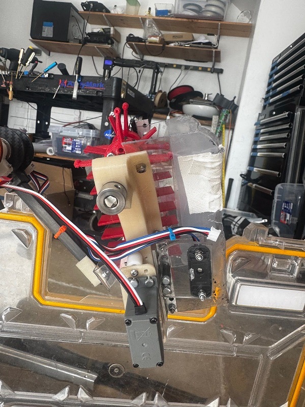

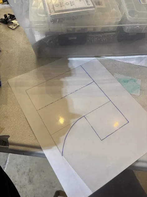
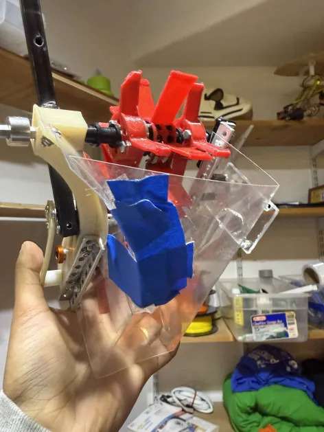
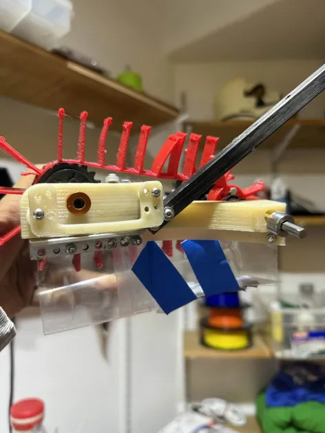
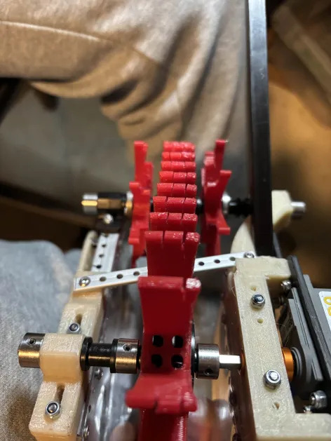
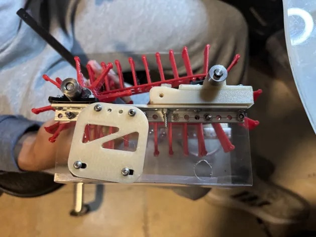
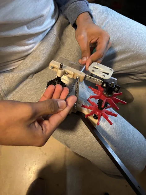
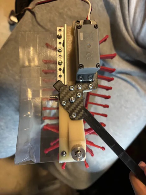
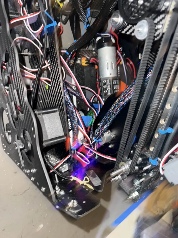
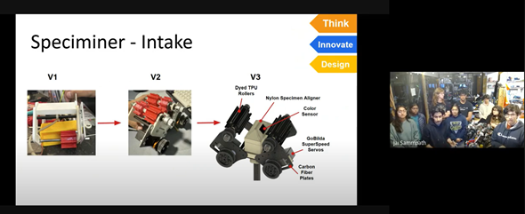
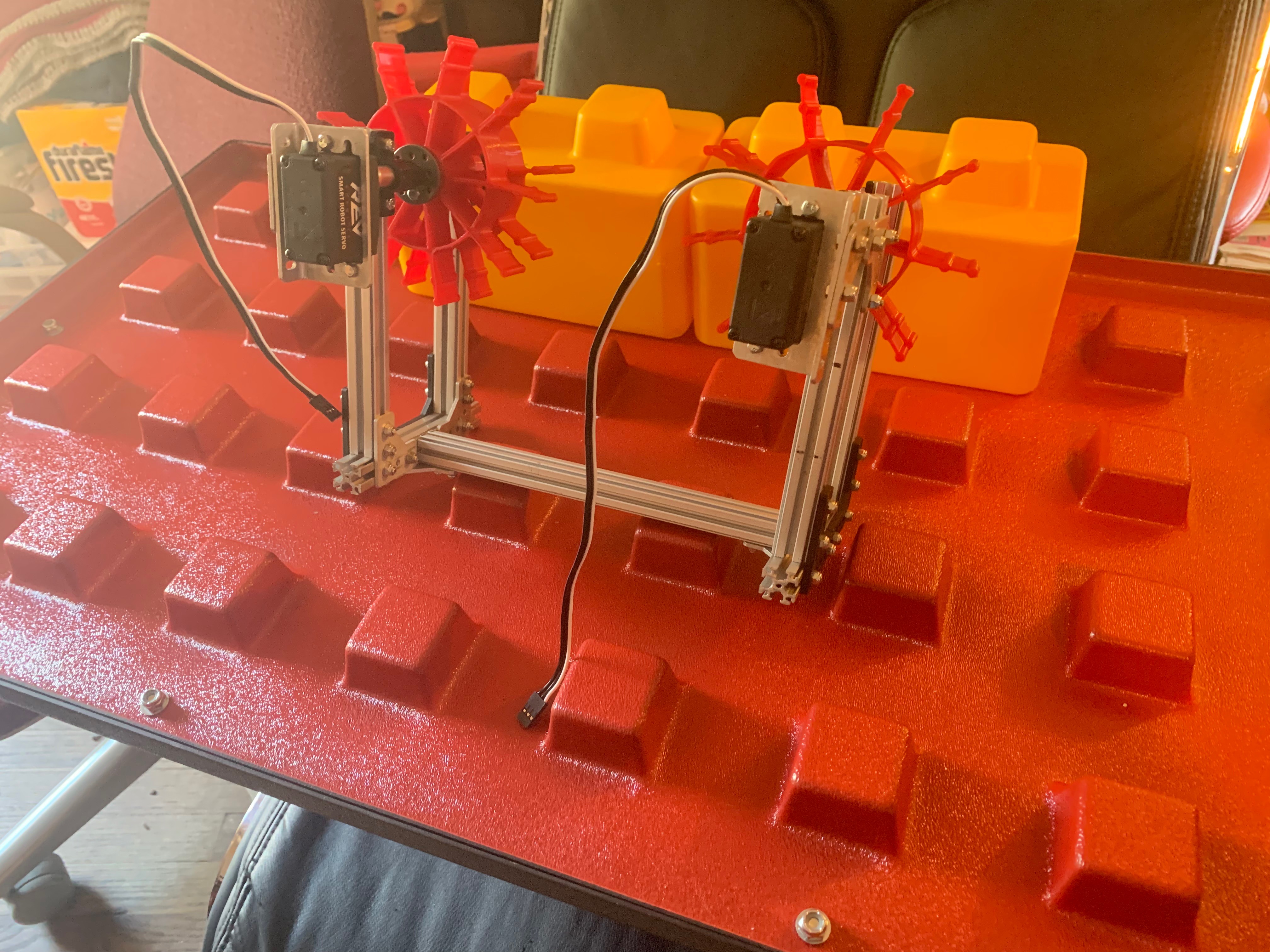
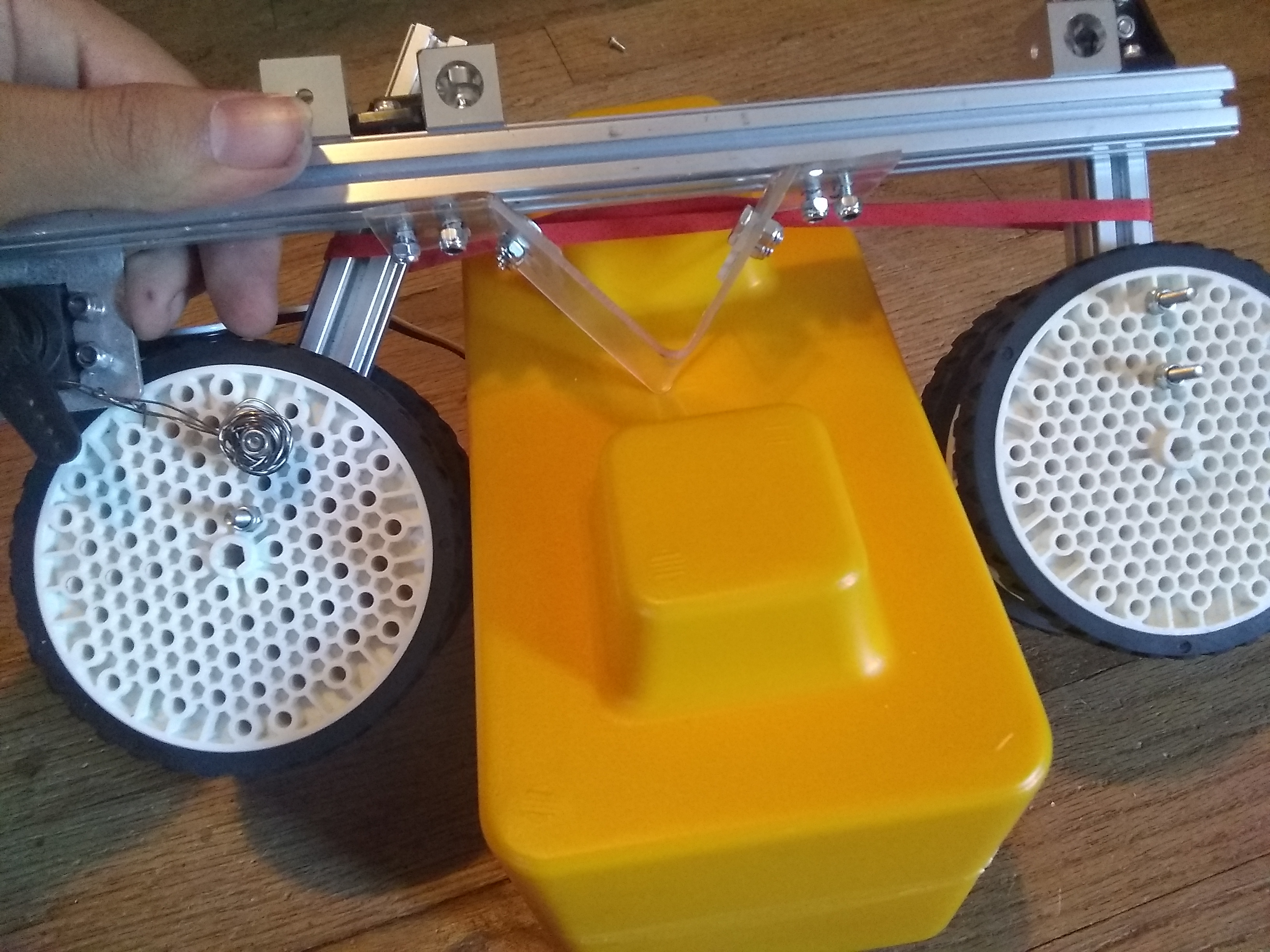
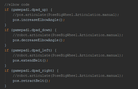
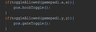
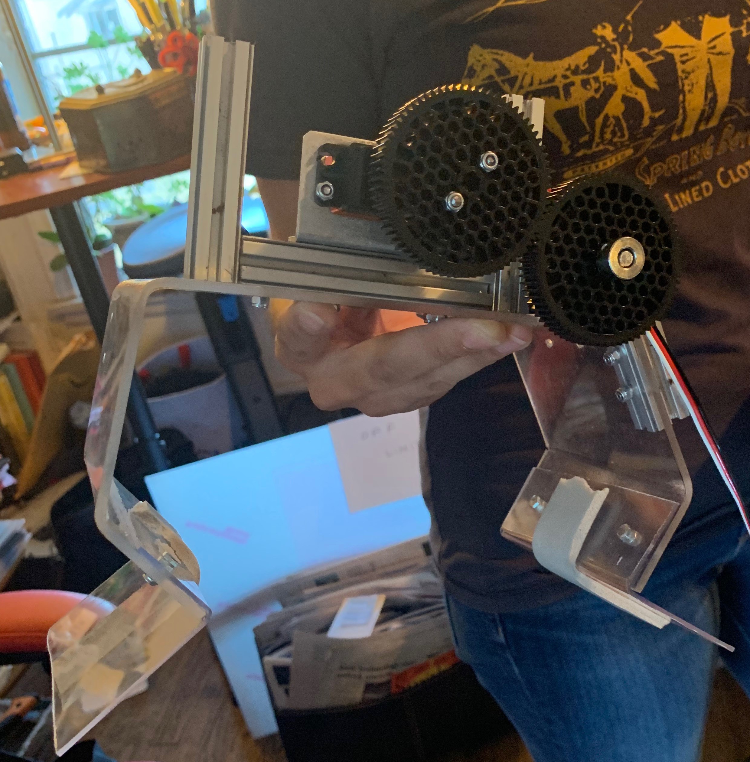
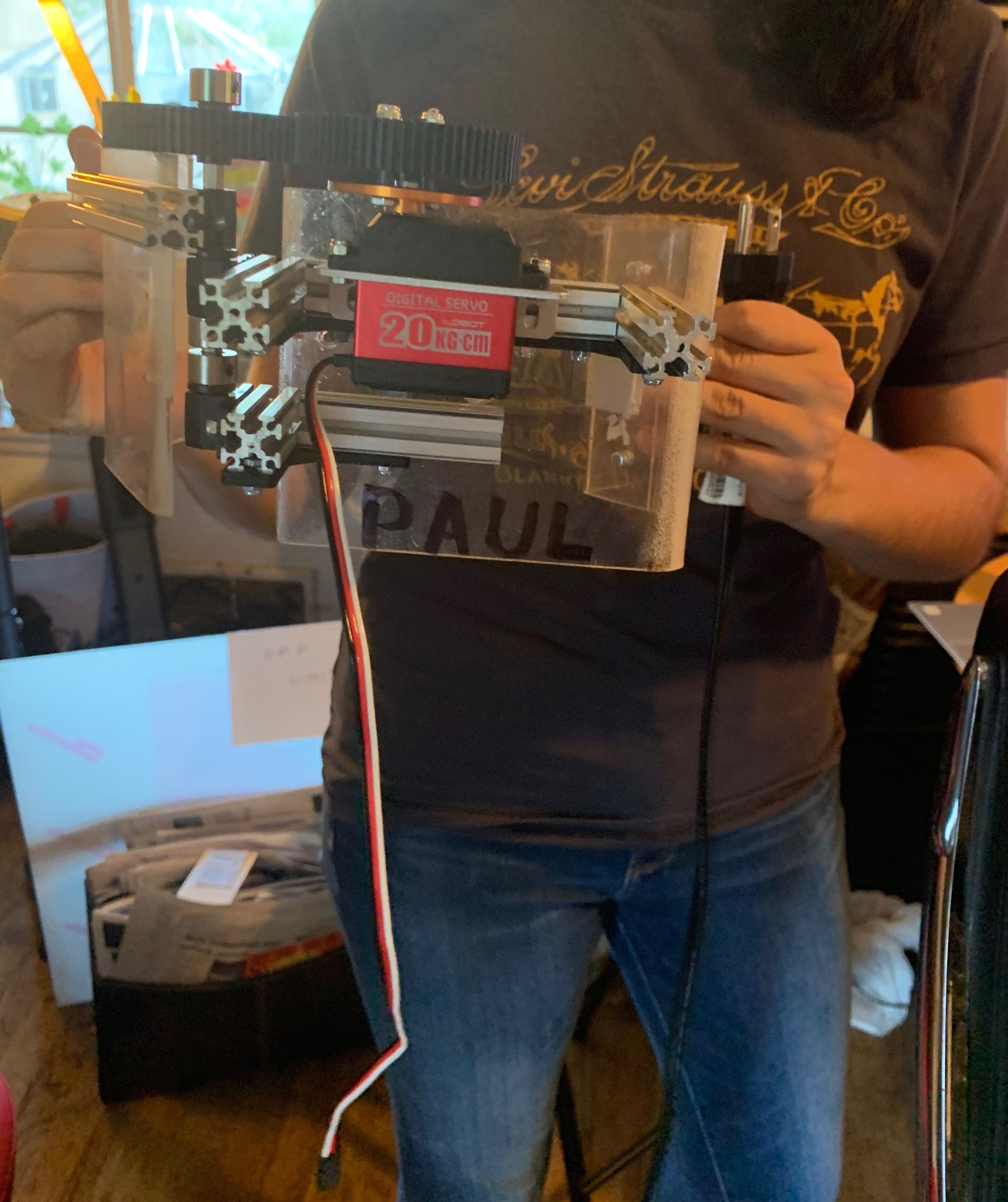
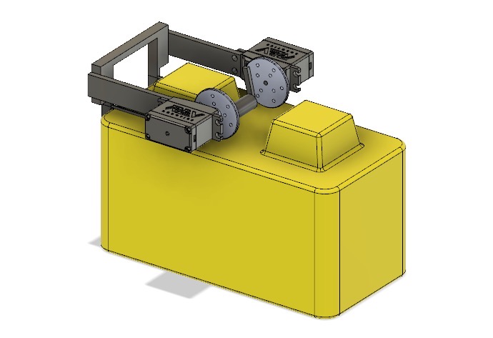
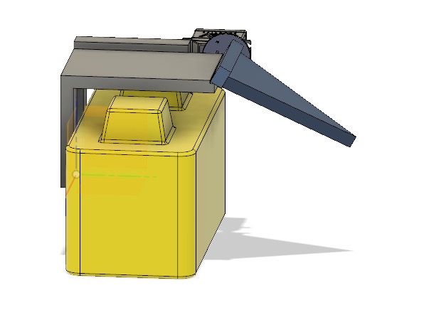
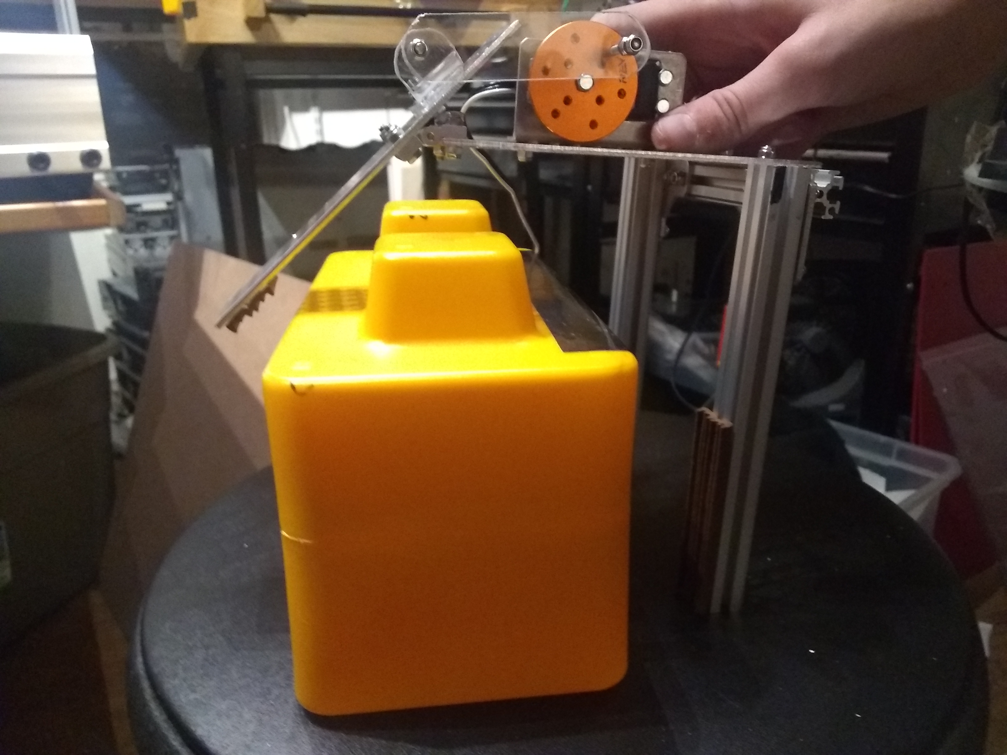
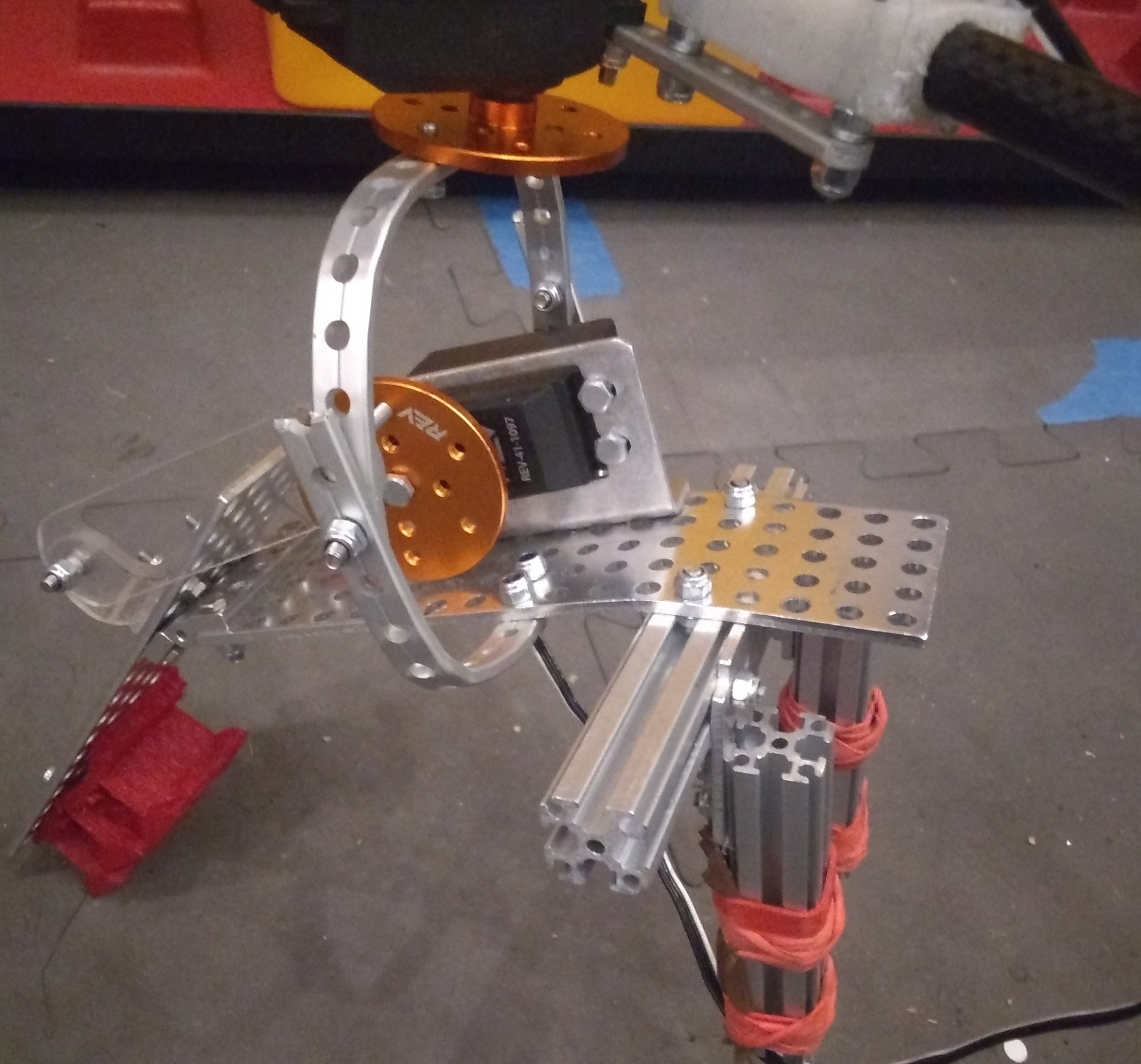
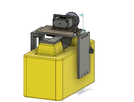
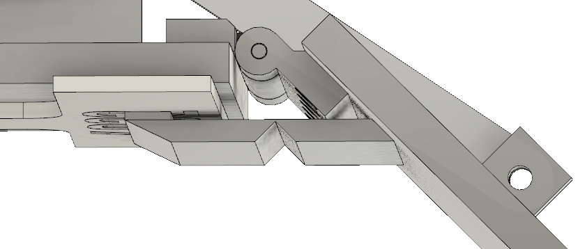
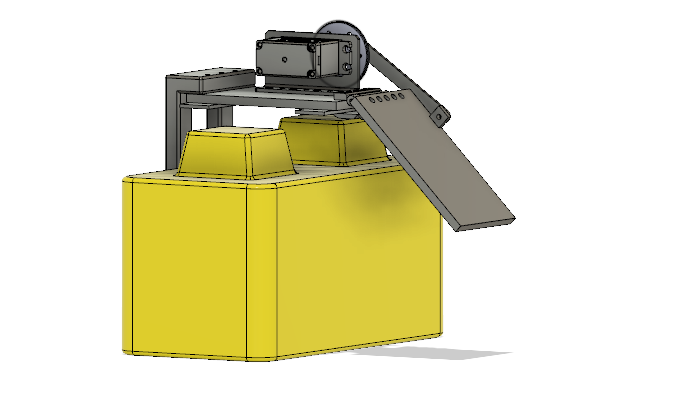
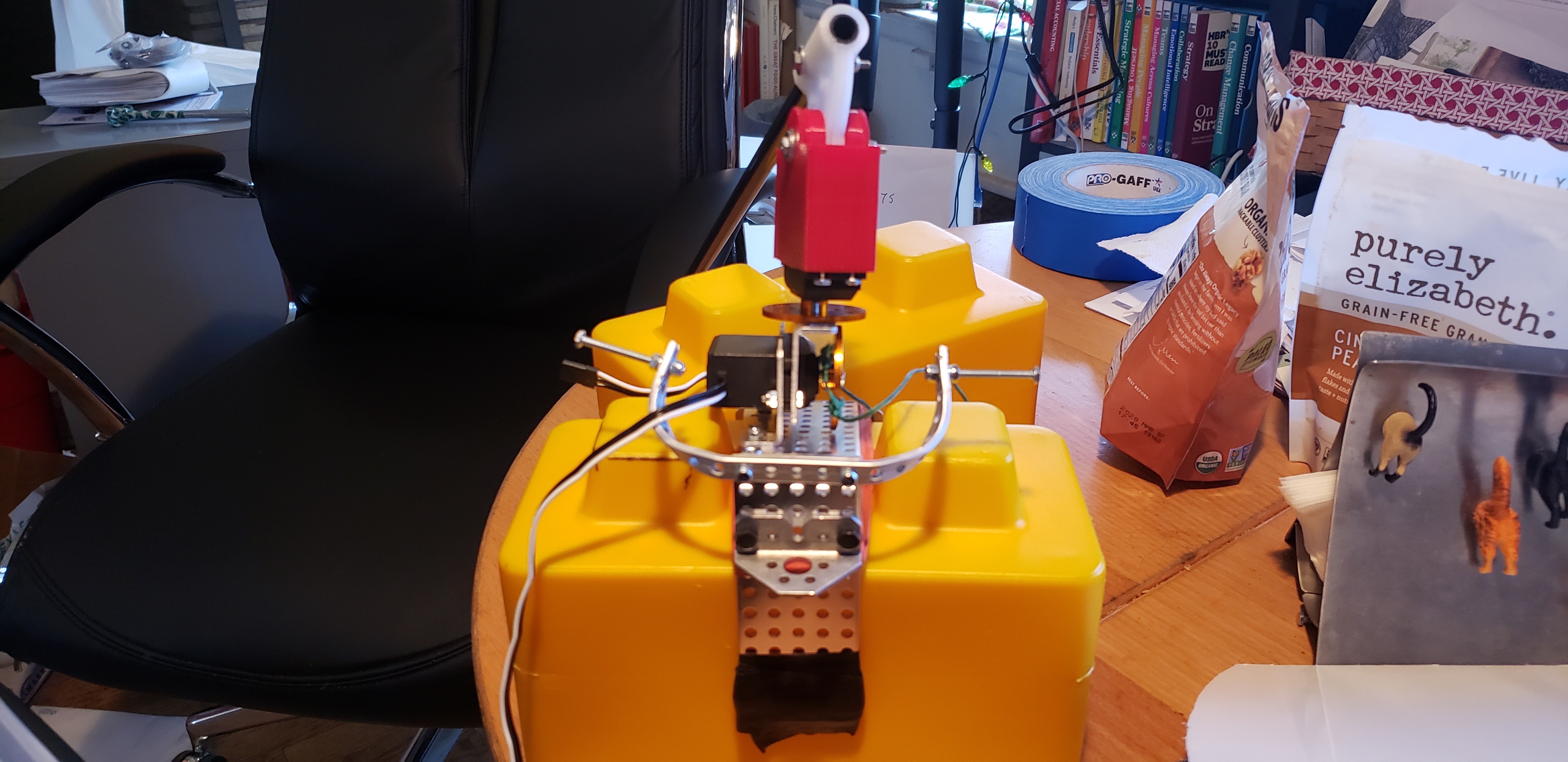
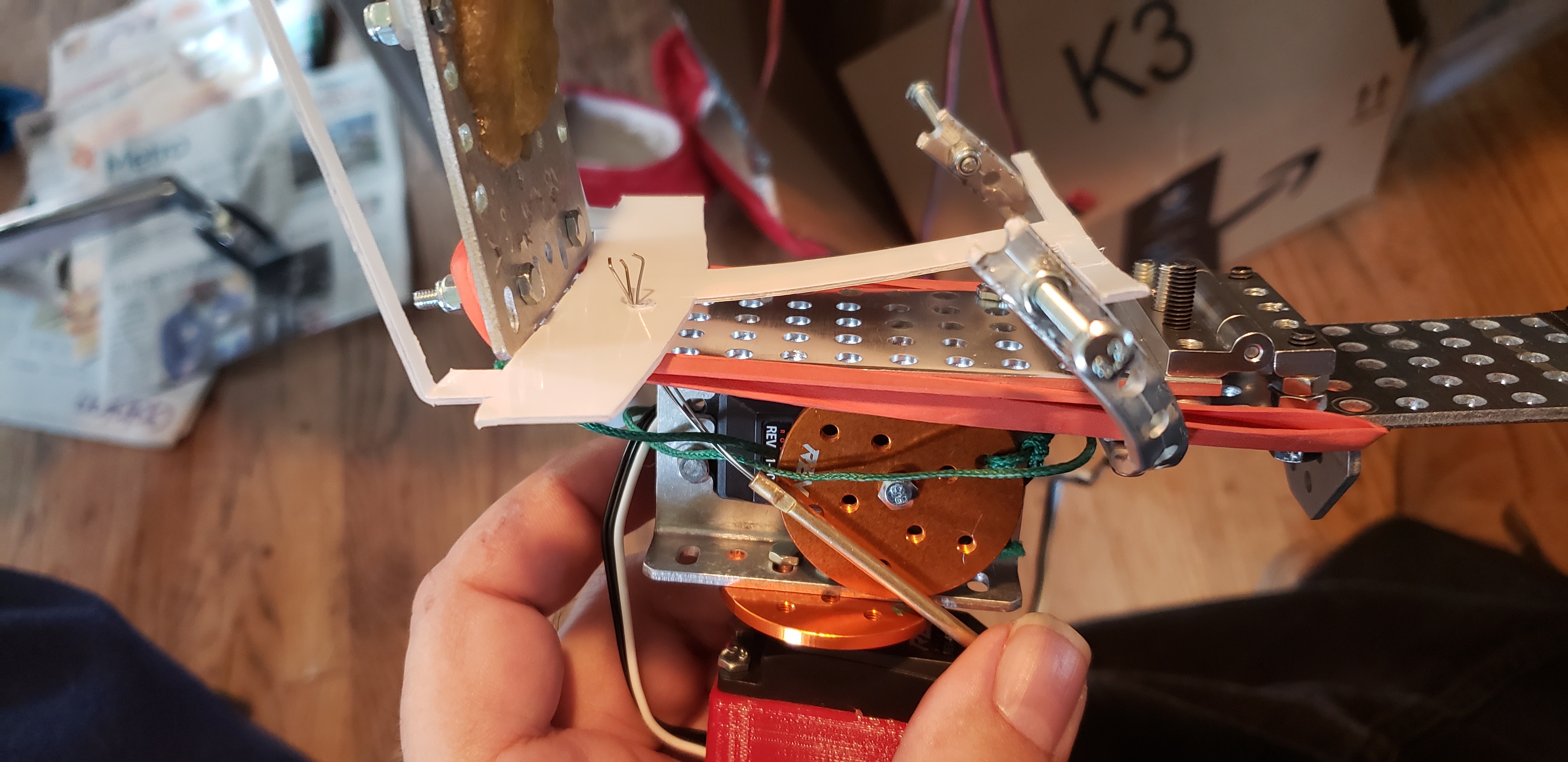
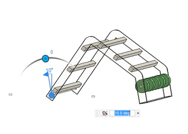
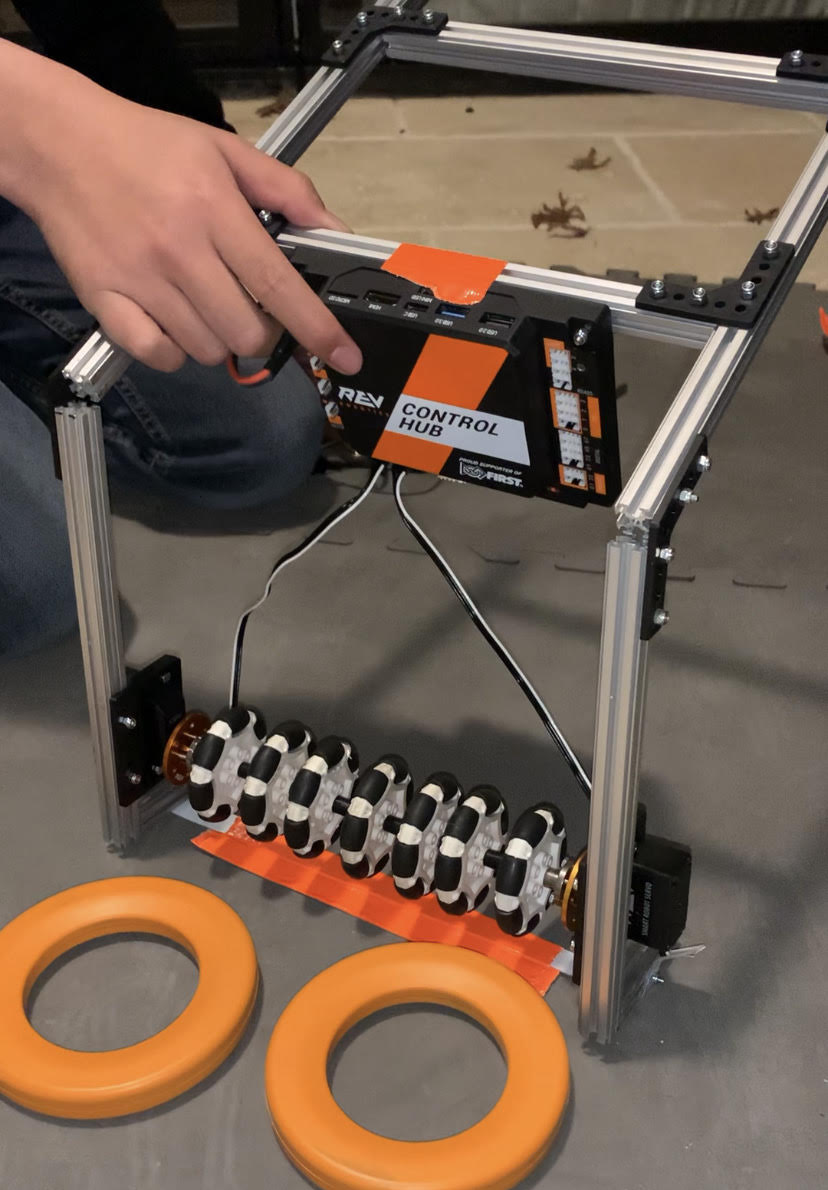
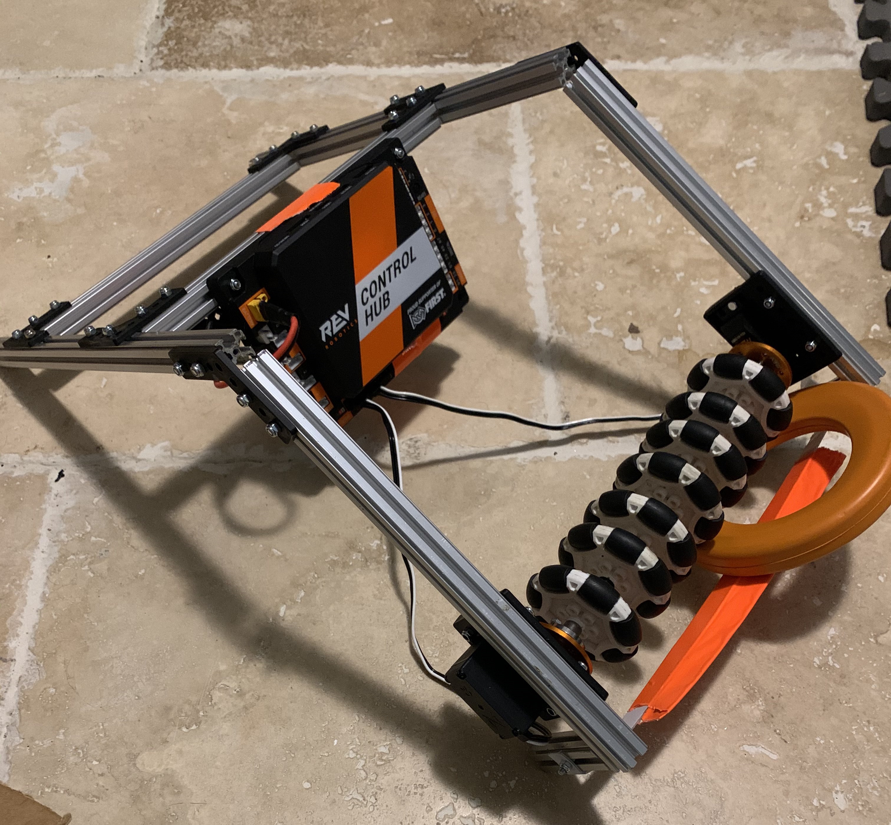
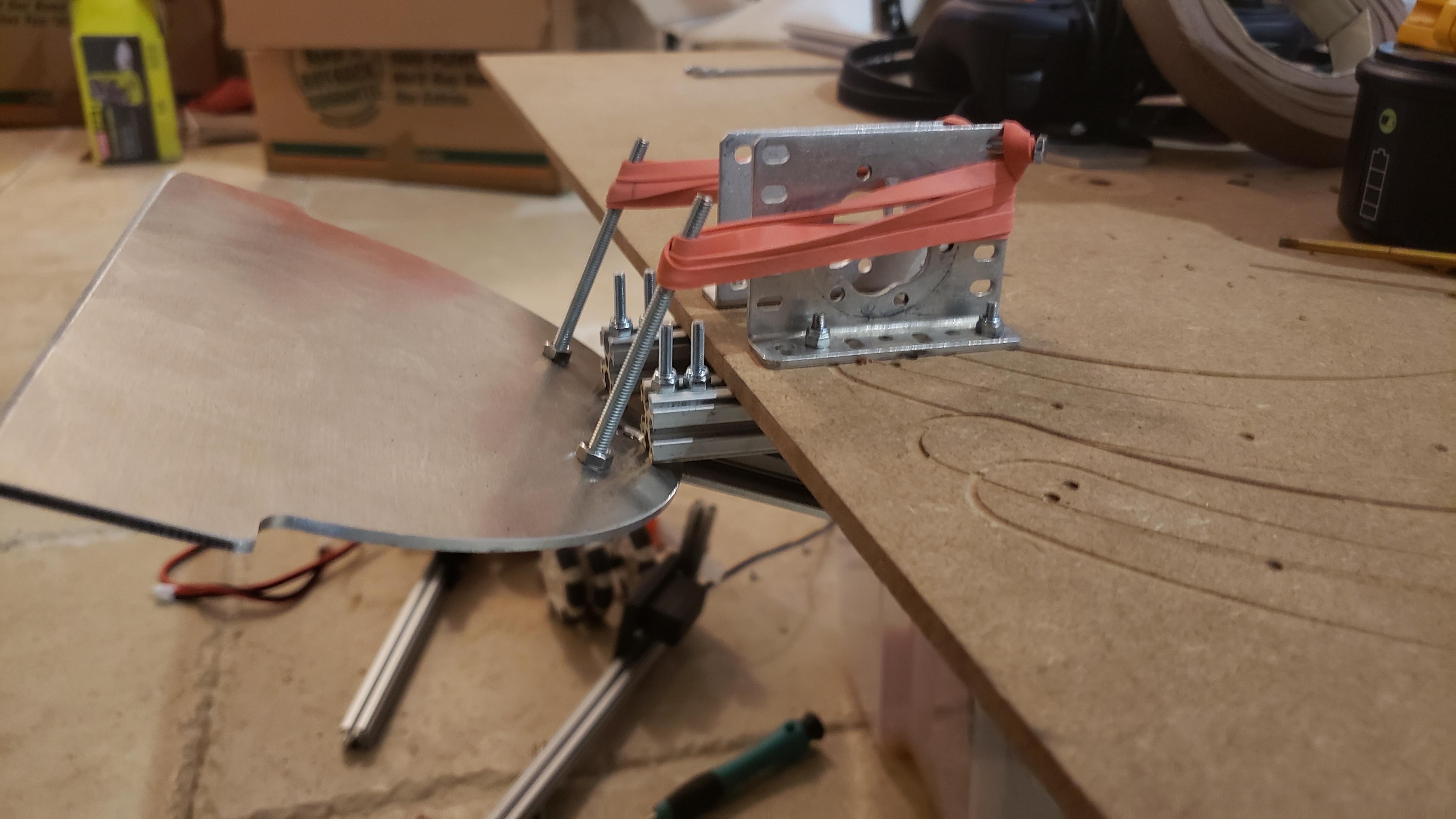
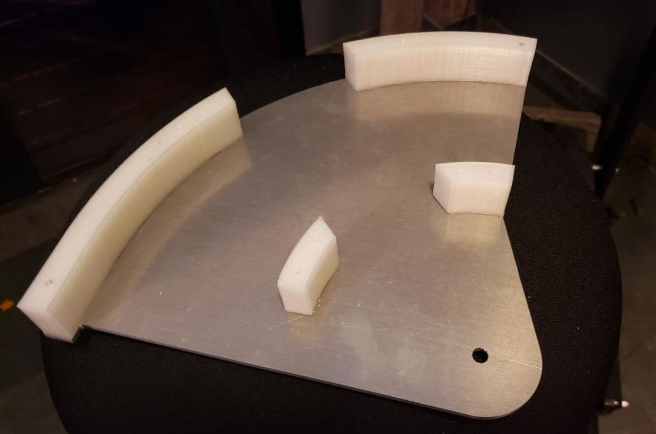
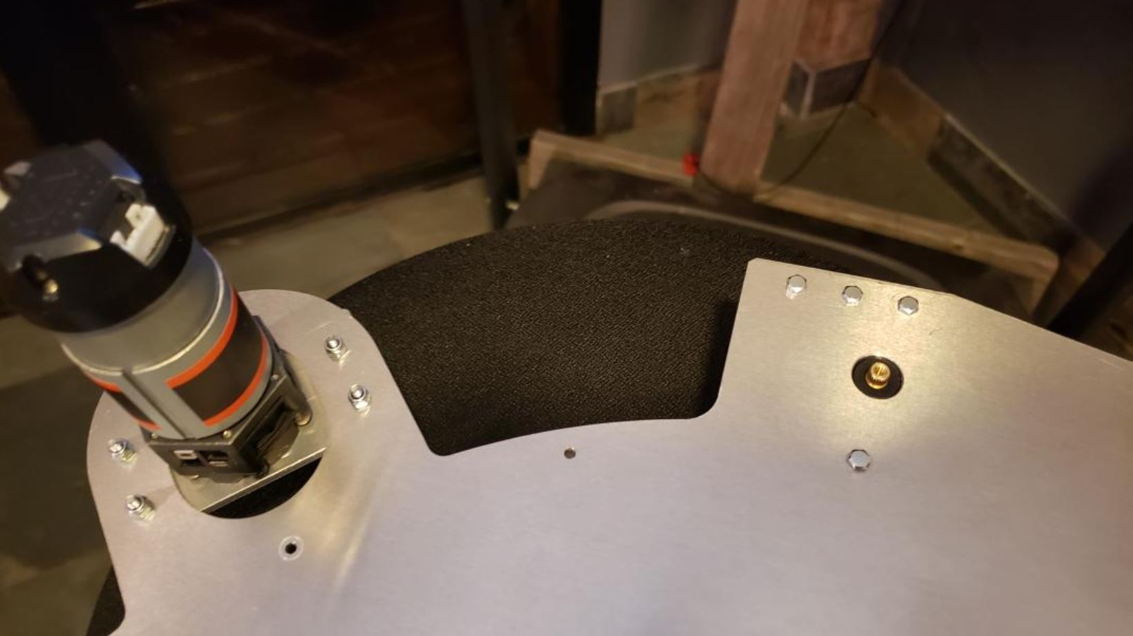
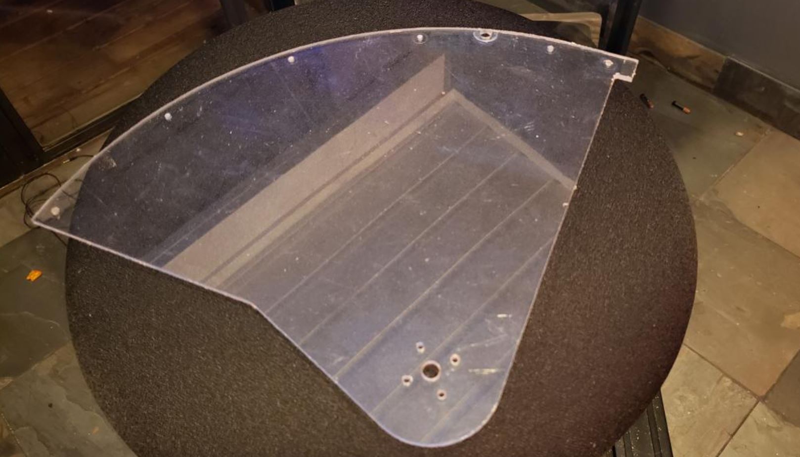
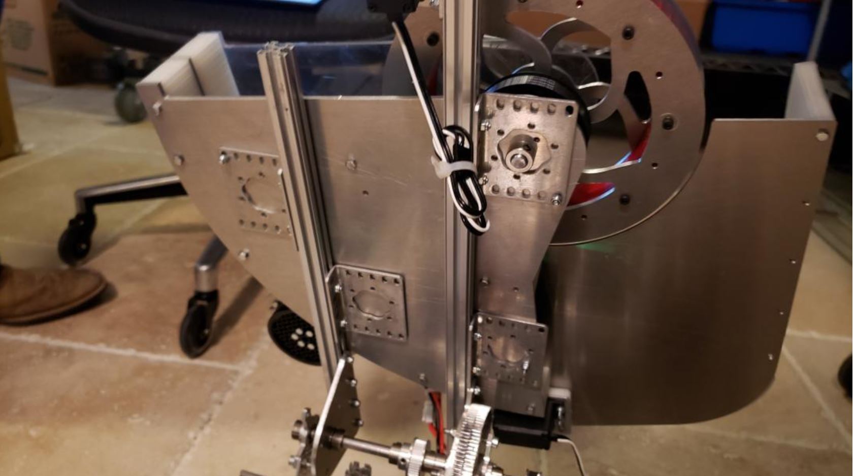
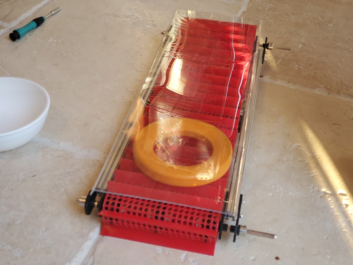
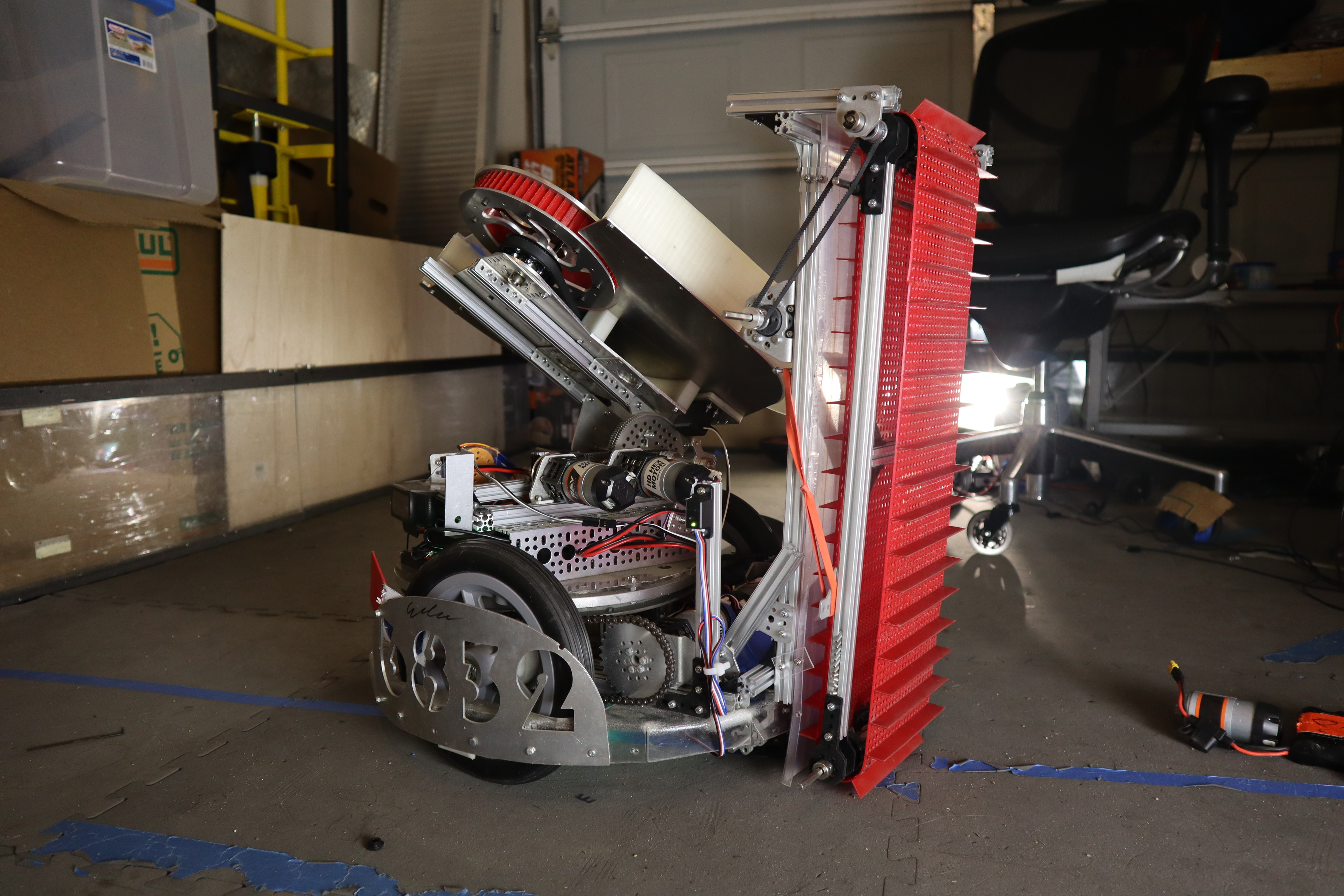
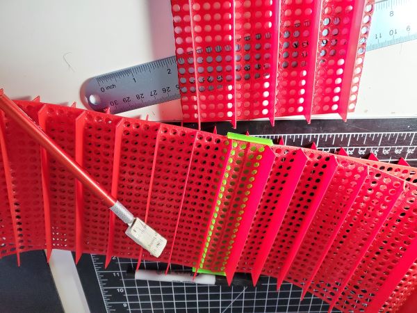
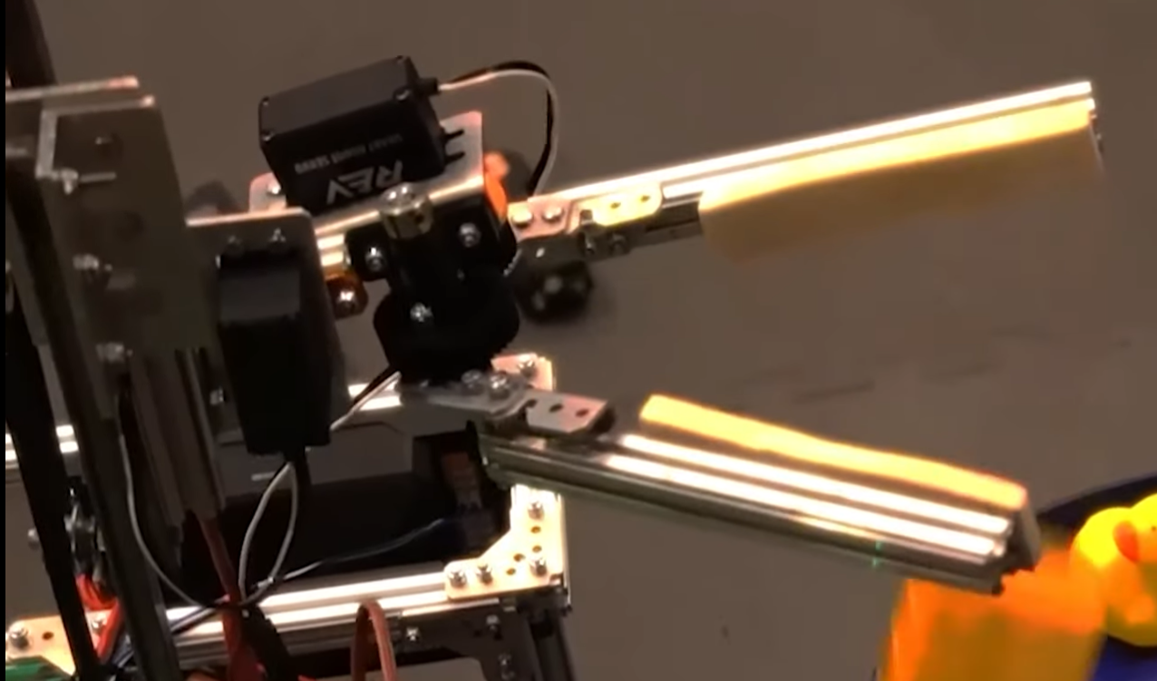
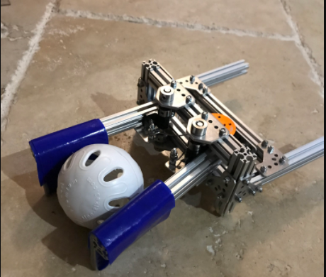
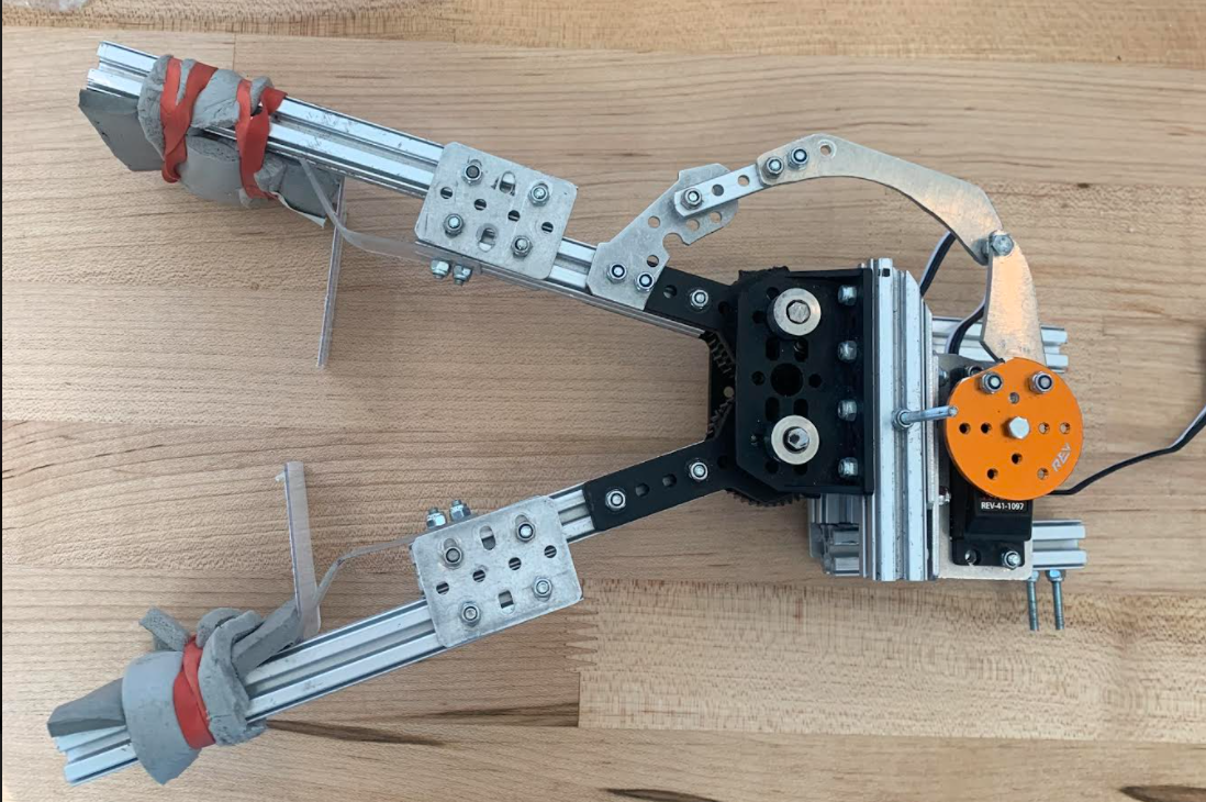
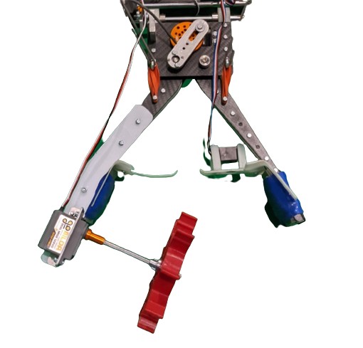
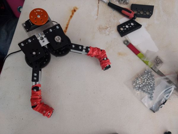
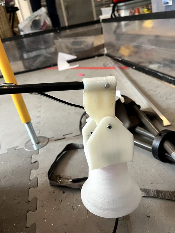
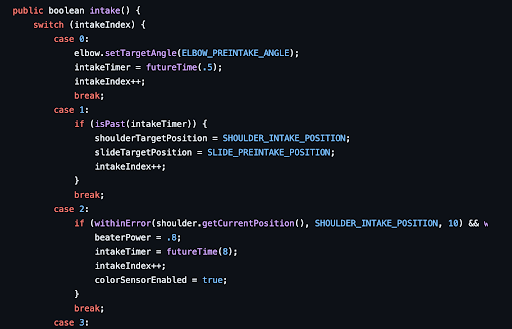 The beginning of our Intake articulation
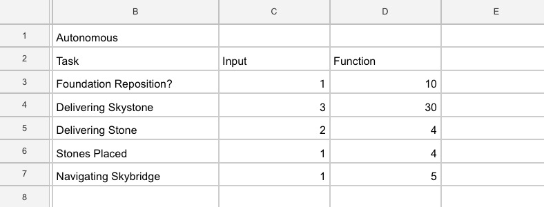
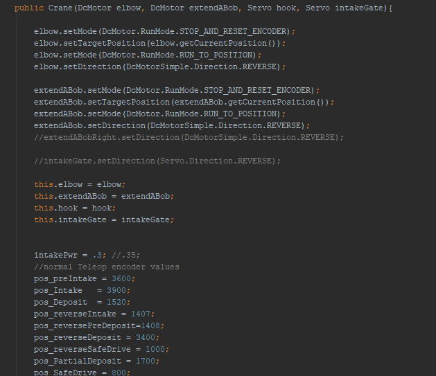
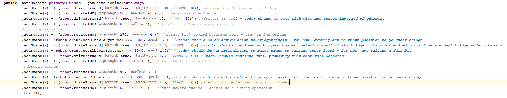
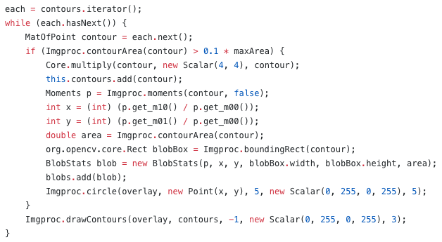
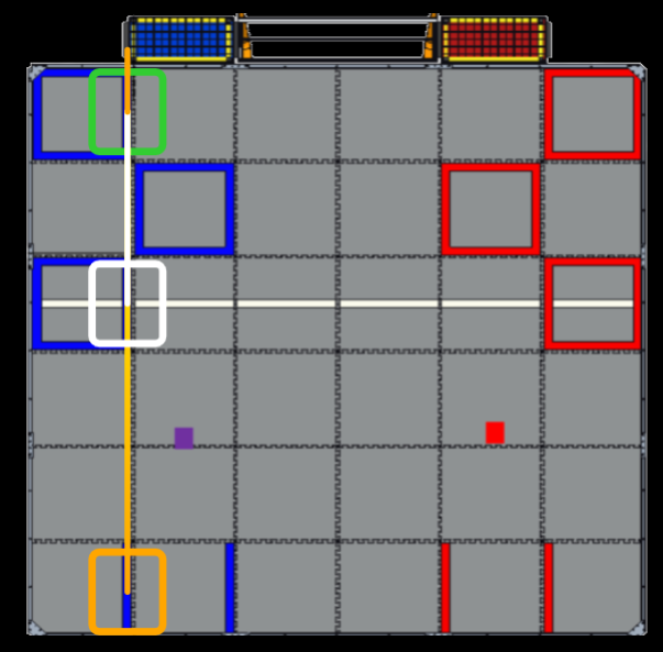
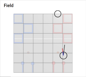
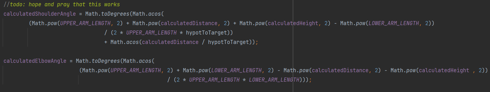
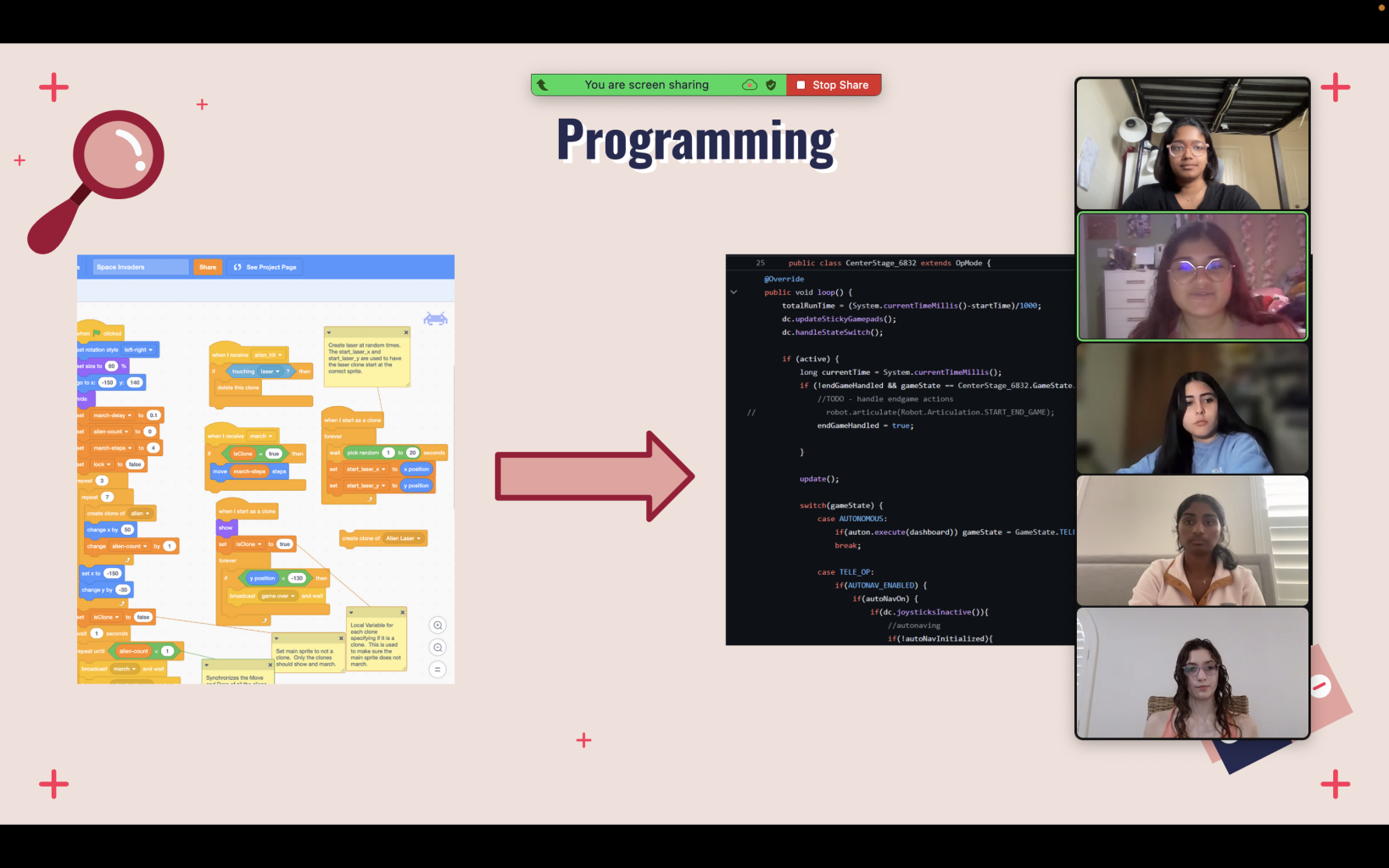
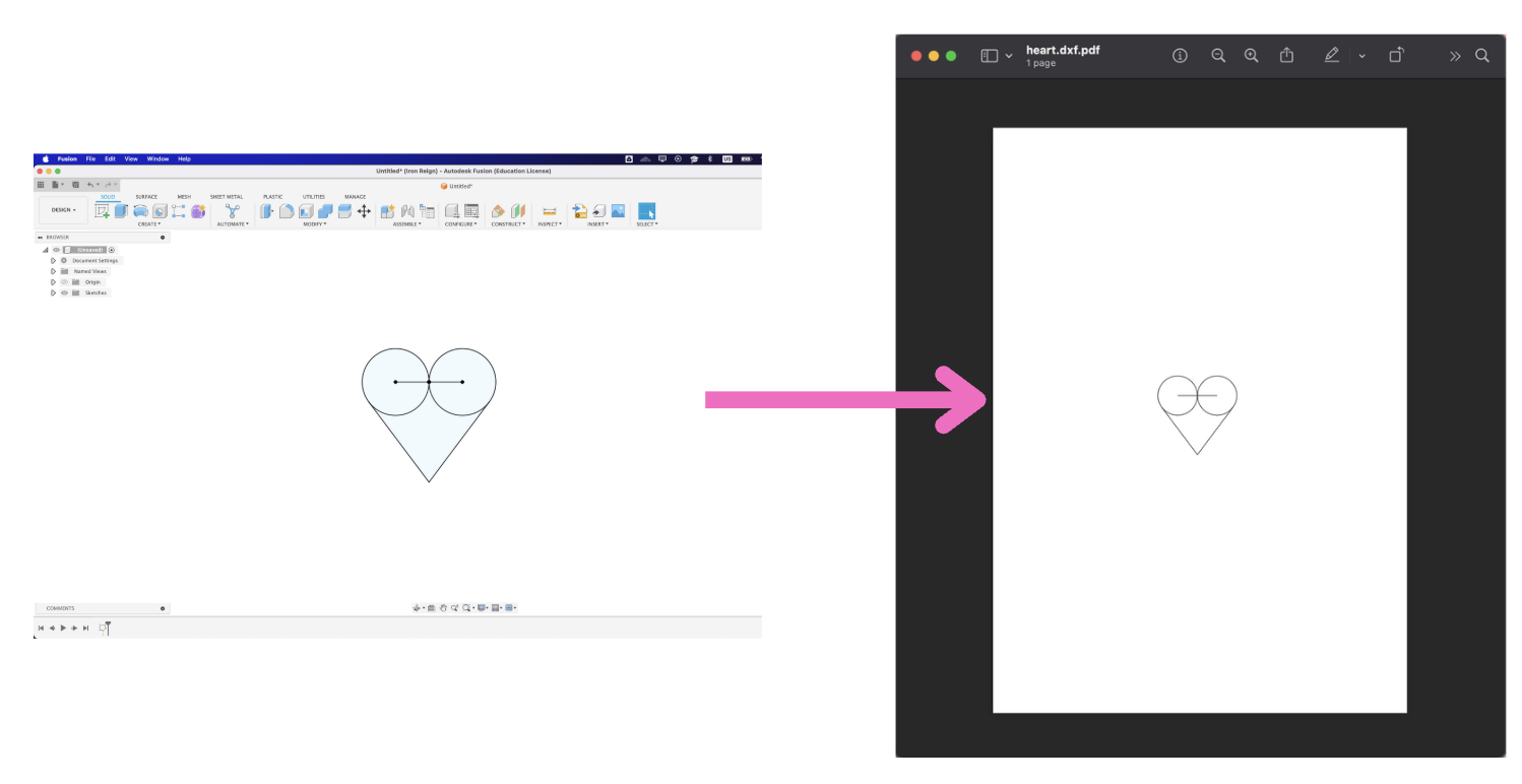
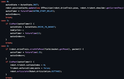 The start of our autonomous state machine