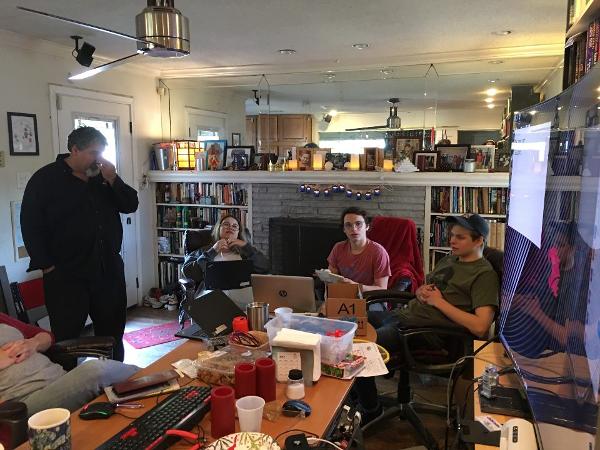
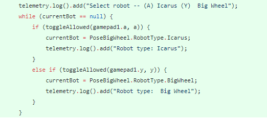
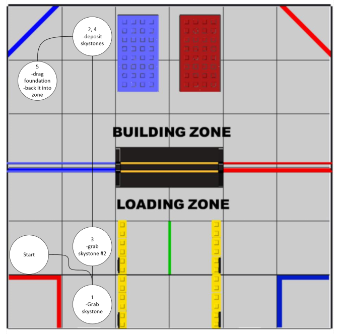
08 Dec 2021
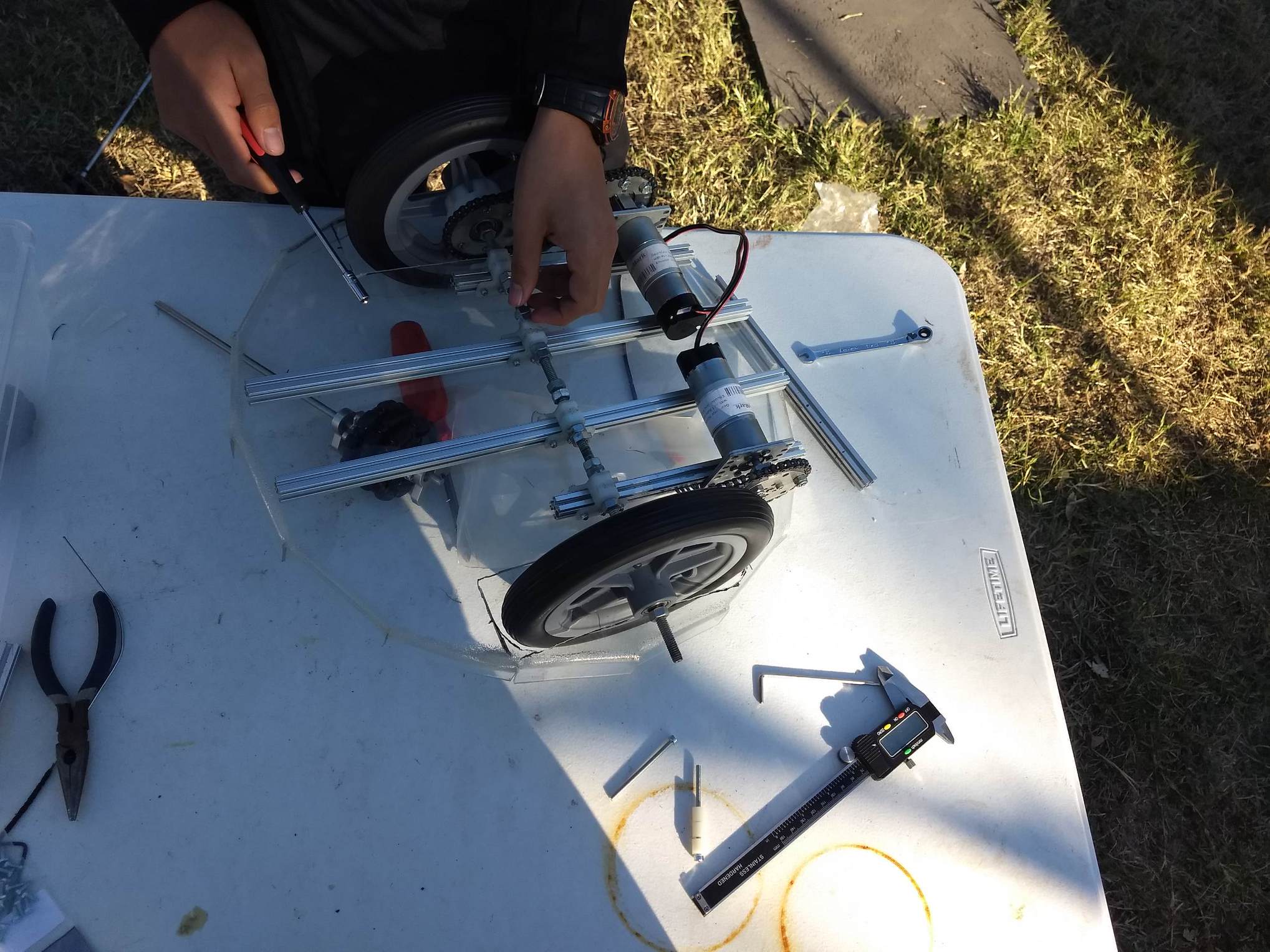
Deriving Inverse Kinematics For The Drivetrain
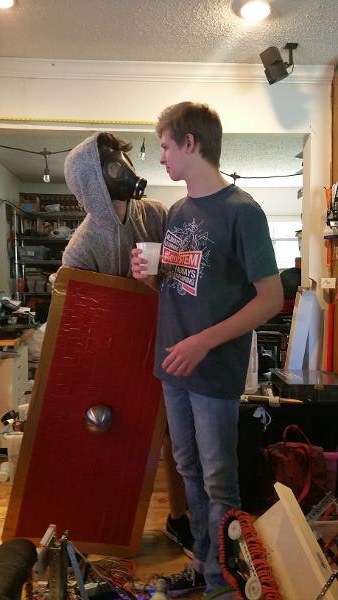
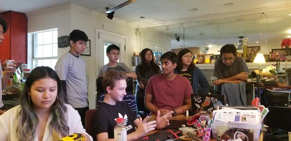
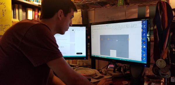
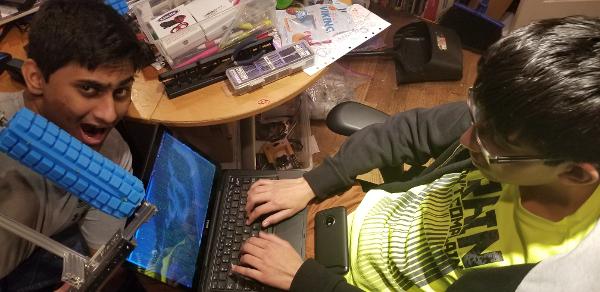
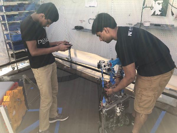
By Mahesh, Cooper, and Ben
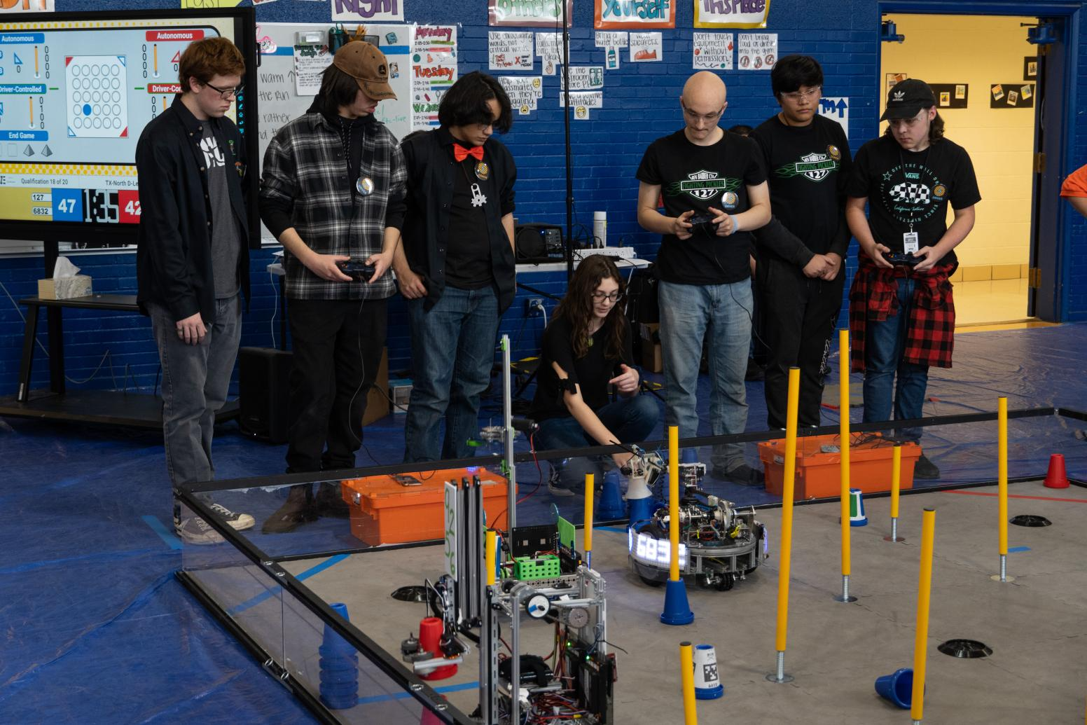
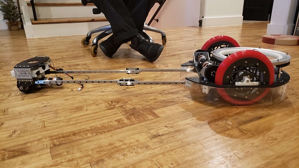
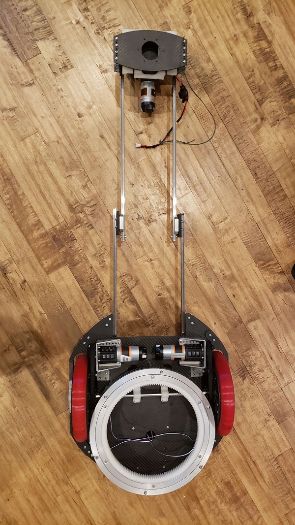
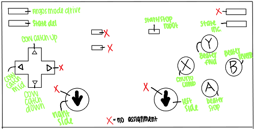
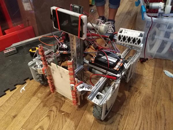
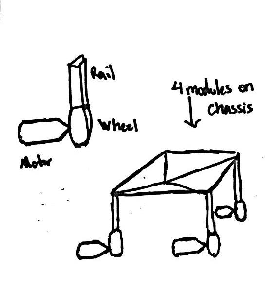
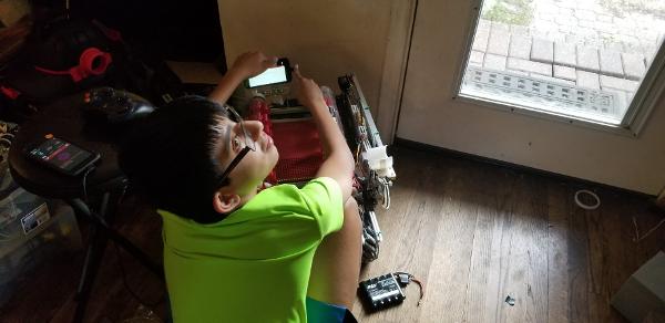
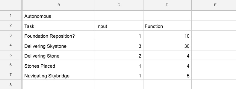
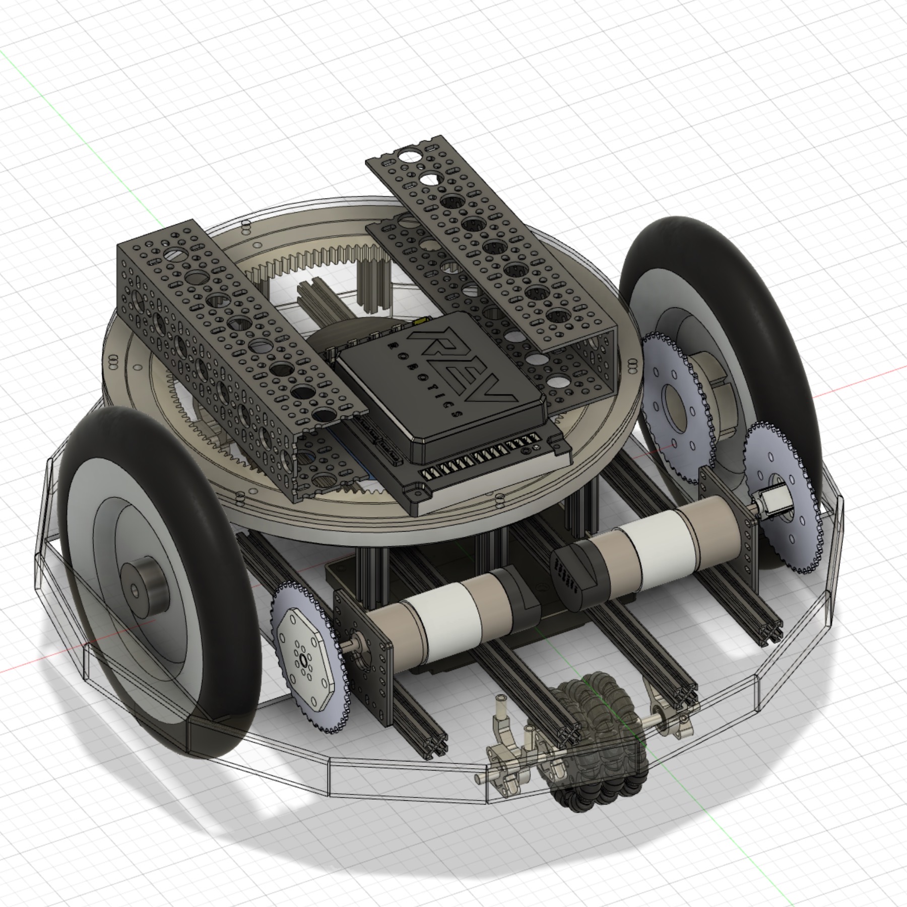
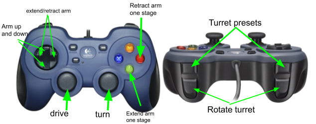
Task: Derive Inverse Kinematics For The Drivetrain
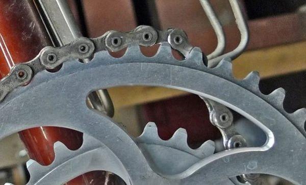
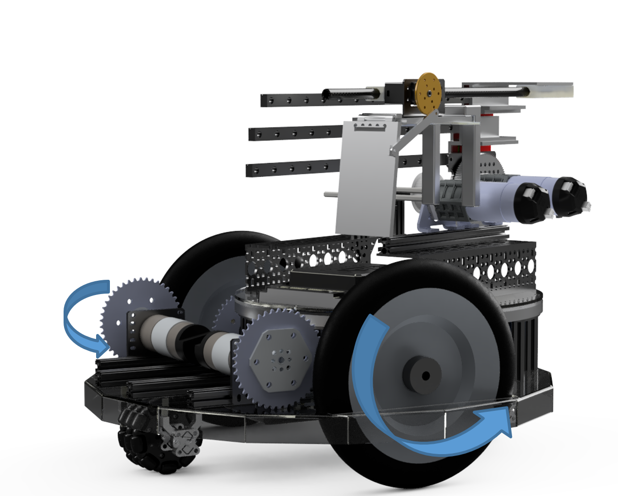
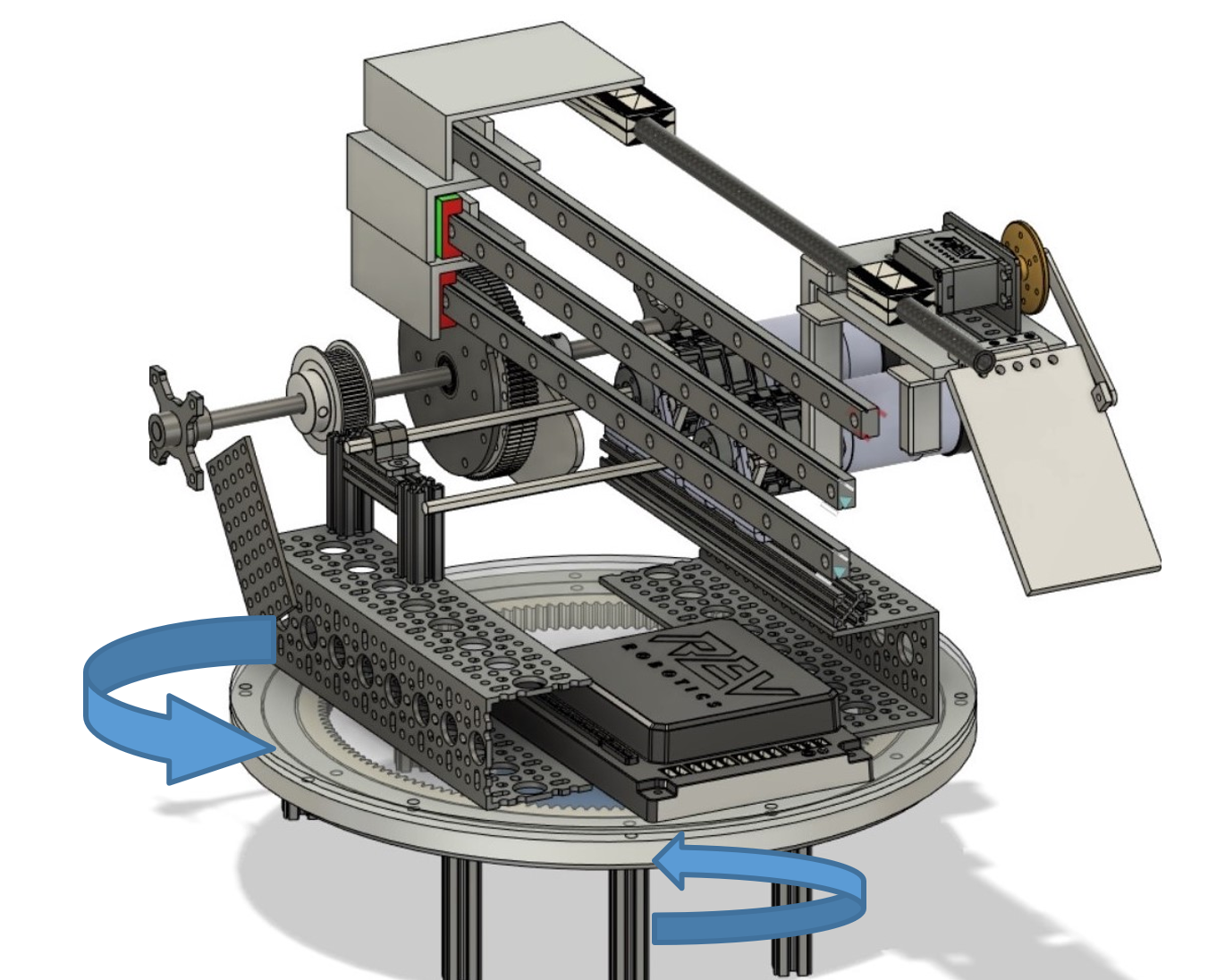
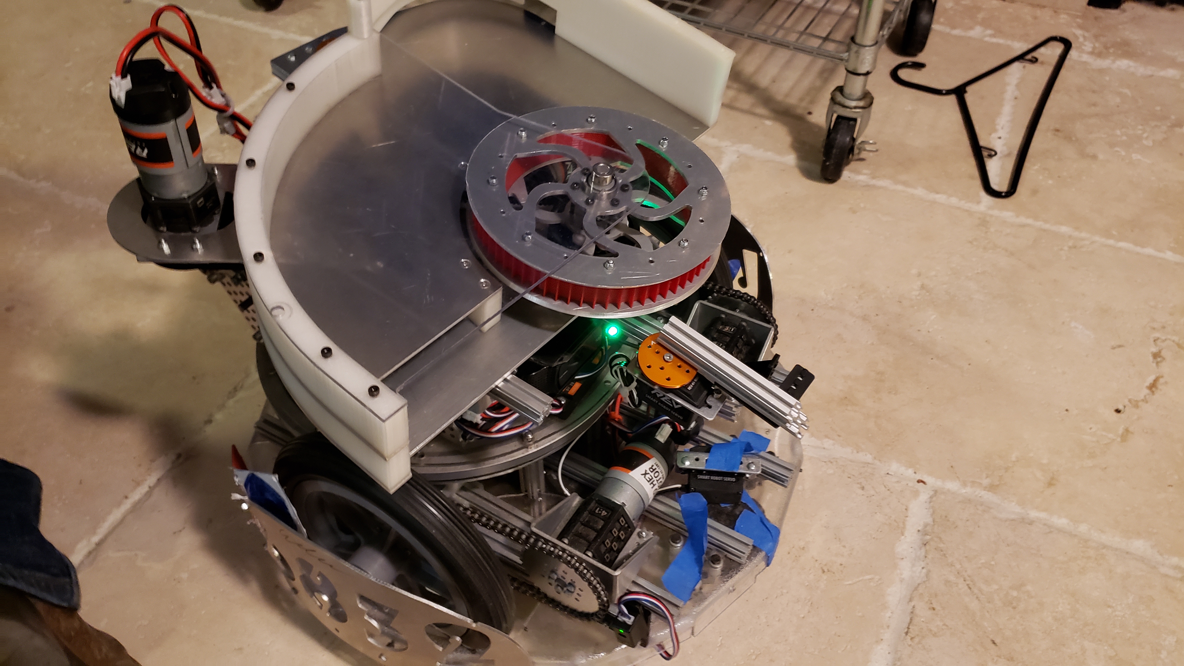
Due to having an unconventential drivetrain consisting of two differental
wheels and a third swerve wheel, it is crucial that we derive the inverse
wheel kinematics early on. These inverse kinematics would convert a
desired linear and angular velocity of the robot to individual wheel
velocities and an angle for the back swerve wheel. Not only would these
inverse kinematics be used during Tele-Op to control the robot through
joystick movements, but it will be useful for getting the robot to travel
at a desired forward velocity and turning rate for autonomous path
following. Either way, deriving basic inverse kinematics for the
drivetrain is a necessity prerequisite for most future programming
endeavors.
More concretely, the problem consists of the following:
Given a desired linear velocity \(v\) and turning rate/angular velocity
\(\omega\), compute the required wheel velocities \(v_l\), \(v_r\), and
\(v_s\), as well as the required swerve wheel angle \(\theta\) to produce
the given inputs. We will define \(v_l\) as the velocity of the left
wheel, \(v_r\) as the velocity of the right wheel, and \(v_s\) as the
velocity of the swerve wheel.
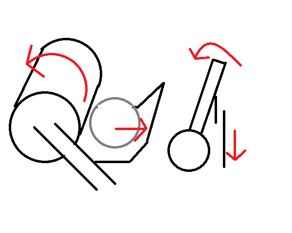
To begin, we can consider the problem from the perspective of the robot
turning with a given turning radius \(r\) with tangent velocity \(v\).
From the equation \(v = \omega r\), we can conclude that \(r =
\frac{v}{\omega}\). Notice that this means when \(\omega = 0\), the radius
blows up to infinity. Intuitively, this makes sense, as traveling in a
straight line (\(\omega = 0\)) is equivalent to turning with an infinite
radius.
The main equation used for inverse wheel kinematics is:
\[\displaylines{\vec{v_b} = \vec{v_a} + \vec{\omega_a} \times \vec{r}}\]
Where \(\vec{v_b}\) is the velocity at a point B, \(\vec{v_a}\) is the
velocity vector at a point A, \(\vec{\omega_a}\) is the angular velocity
vector at A, and \(\vec{r}\) is the distance vector pointing from A to B.
The angular velocity vector will point out from the 2-D plane of the robot
in the third, \(\hat{k}\), axis (provable using the right-hand rule).
But why exactly does this equation work? What connection does the cross
product have with deriving inverse kinematics? In the following section,
the above equation will be proven. See section 1.1 to skip past the proof.
To understand the equation, we start by considering a point A rotating
around aother point B with turn radius vector \(\hat{r}\) and tangent
velocity \(\vec{v}\).
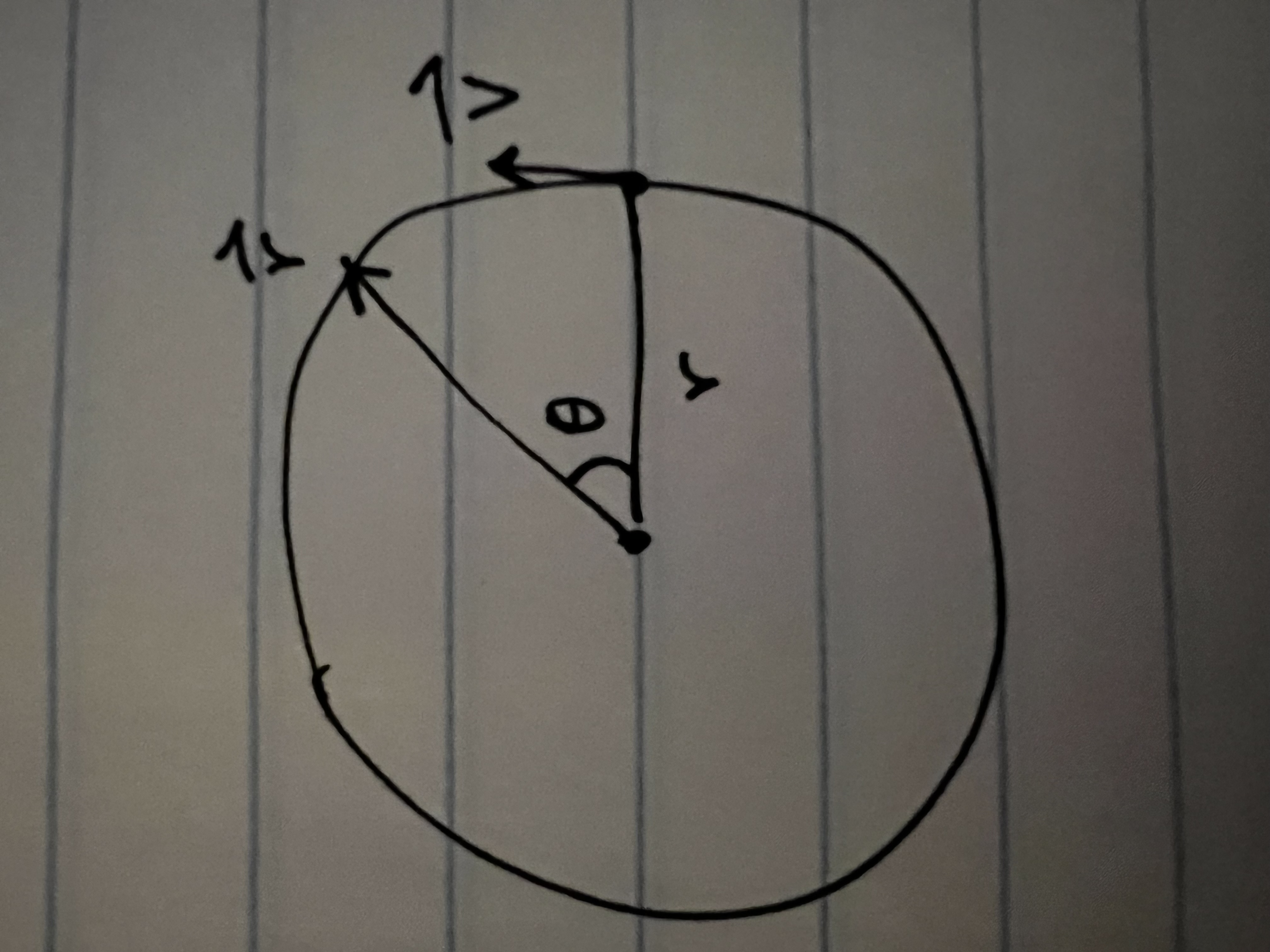
For an angle \(\theta\) around the x-axis, the position vector \(\vec{s}\)
can be defined as the following:
\[\displaylines{\vec{s} = r(\hat{i}\cos\theta + \hat{j}\sin\theta) }\]
by splitting the radius vector into its components and recombining them.
To arrive at a desired equation for \(\vec{v}\), we will have to
differentiate \(\vec{r}\) with respect to time. By the chain rule:
\[\displaylines{\vec{v} = \frac{d\vec{s}}{dt} = \frac{d\vec{s}}{d\theta}
\cdot \frac{d\theta}{dt}}\]
The appropriate equations for \(\frac{d\vec{s}}{d\theta}\) and
\(\frac{d\theta}{dt}\) can then be multiplied to produce the desired
\(\vec{v}\):
\[\displaylines{\frac{d\vec{s}}{d\theta} = \frac{d}{d\theta} \vec{s} =
\frac{d}{d\theta} r(\hat{i}\cos\theta + \hat{j}\sin\theta) =
r(-\hat{i}sin\theta + \hat{j}cos\theta) \\ \frac{d\theta}{dt} = \omega \\
\vec{v} = \frac{d\vec{s}}{dt} = \frac{d\vec{s}}{d\theta} \cdot
\frac{d\theta}{dt} = r(-\hat{i}sin\theta + \hat{j}cos\theta) \cdot \omega
\mathbf{= \omega r(-\hat{i}sin\theta + \hat{j}cos\theta)} }\]
Now that we have an equation for \(\vec{v}\) defined in terms of
\(\omega\), \(r\), and \(\theta\), if we can derive the same formula using
\(\vec{\omega} \times \vec{r}\), we will have proved that \(\vec{v} =
\frac{d\vec{s}}{dt} = \vec{\omega} \times \vec{r}\)
To begin, we will define the following \(\vec{\omega}\) and \(\vec{r}\):
\[\displaylines{ \vec{\omega} = \omega \hat{k} = \begin{bmatrix}0 & 0 &
\omega\end{bmatrix} \\ \vec{r} = r(\hat{i}cos\theta + \hat{j}sin\theta) =
\hat{i}rcos\theta + \hat{j}rsin\theta = \begin{bmatrix}rcos\theta &
rsin\theta & 0\end{bmatrix} }\]
Then, by the definition of a cross product:
\[\displaylines{ \vec{\omega} \times \vec{r} = \begin{vmatrix} \hat{i} &
\hat{j} & \hat{k} \\ 0 & 0 & \omega \\ rcos\theta & rsin\theta & 0
\end{vmatrix} \\ = \hat{i}\begin{vmatrix} 0 & \omega \\ rsin\theta &
0\end{vmatrix} - \hat{j}\begin{vmatrix} 0 & \omega \\ rcos\theta &
0\end{vmatrix} + \hat{k}\begin{vmatrix} 0 & 0 \\ rcos\theta &
rsin\theta\end{vmatrix} \\ = \hat{i}(-\omega rsin\theta) - \hat{j}(-\omega
rcos\theta) + \hat{k}(0) \\ \mathbf{= \omega r(-\hat{i}sin\theta +
\hat{j}cos\theta)}}\]
Since the same resulting equation, \(\omega r(-\hat{i}sin\theta +
\hat{j}cos\theta)\), is produced from evaluating the cross product of
\(\vec{\omega}\) and \(\vec{r}\) and by evaluating
\(\frac{d\vec{s}}{dt}\), we can conclude that \(\vec{v} = \vec{\omega}
\times \vec{r}\)
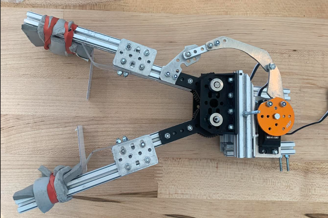
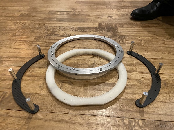
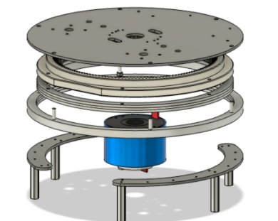
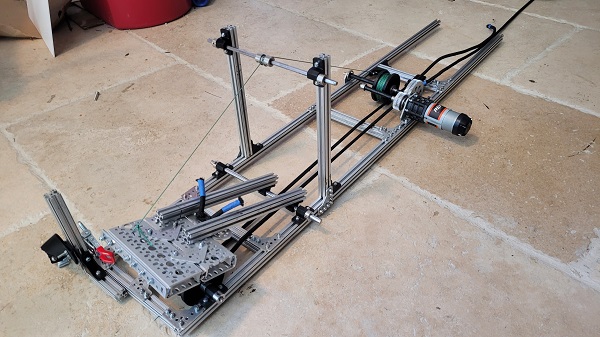
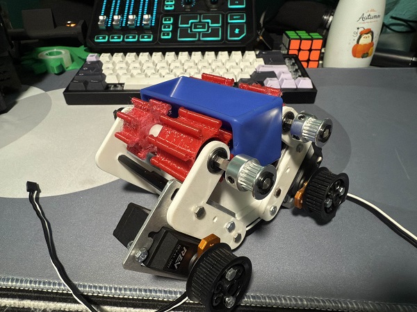
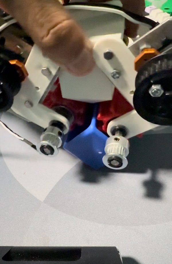
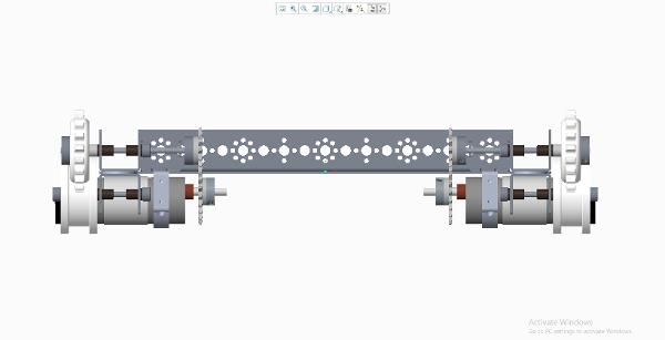
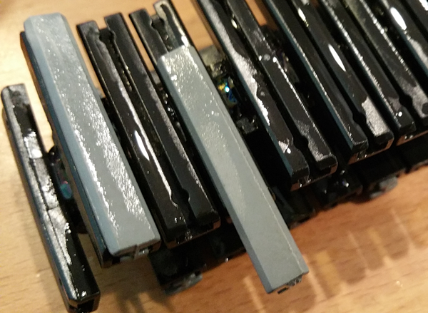
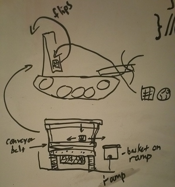
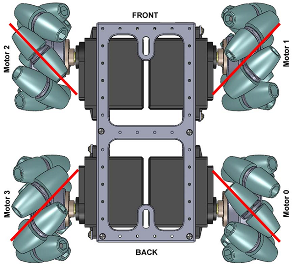
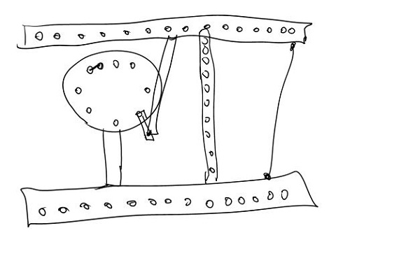
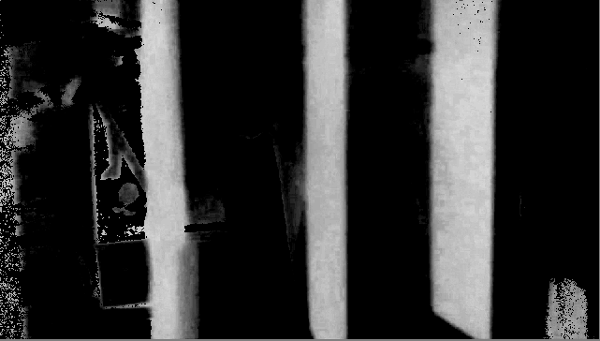
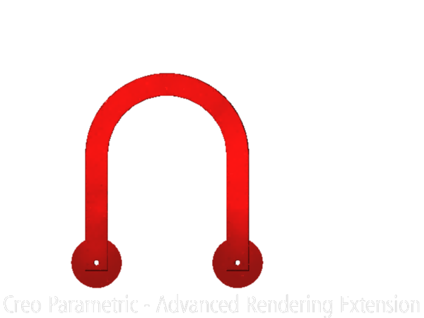
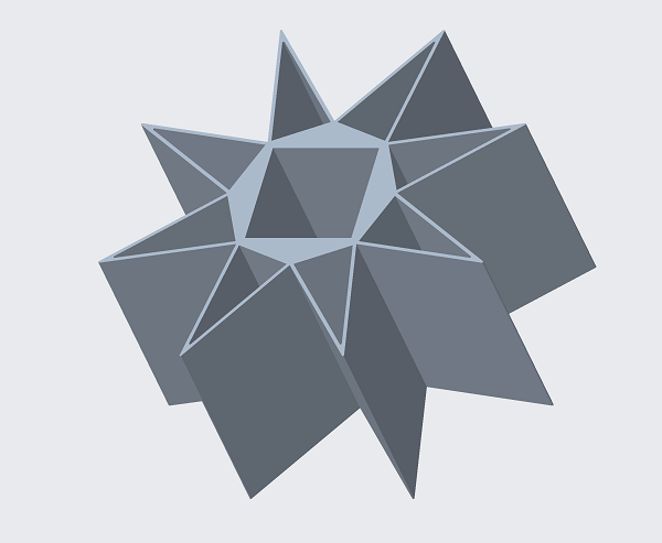
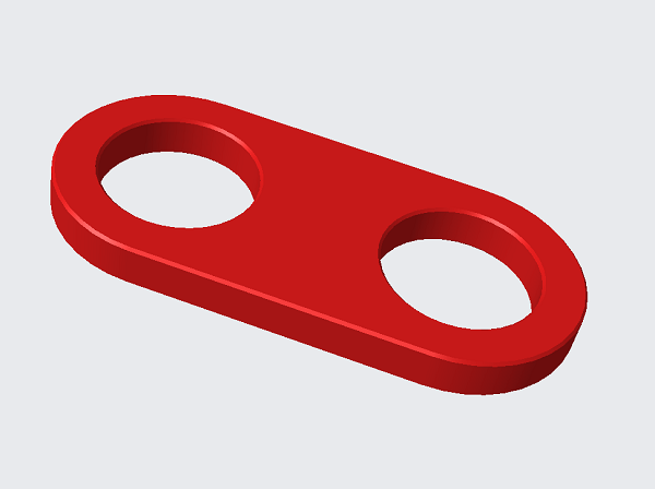
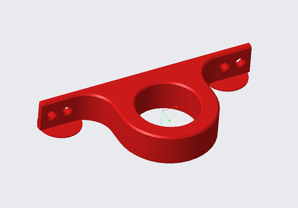
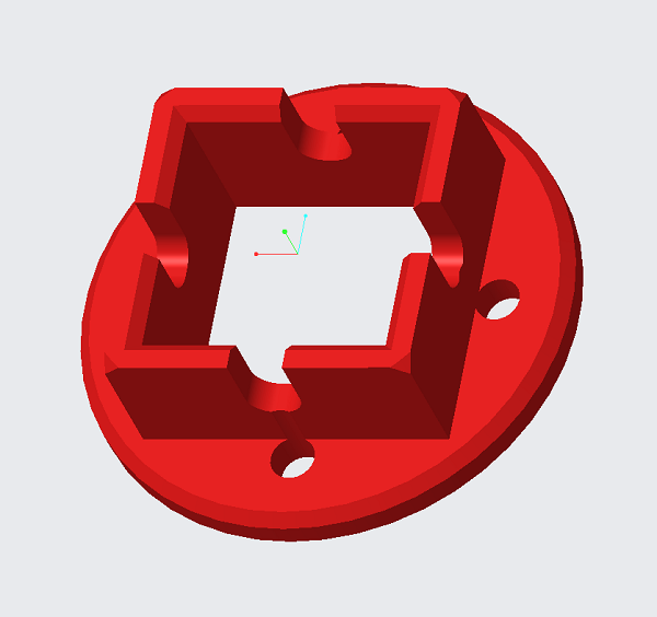
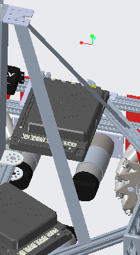
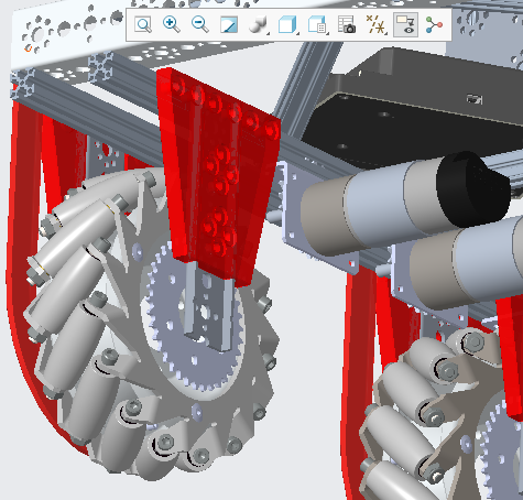
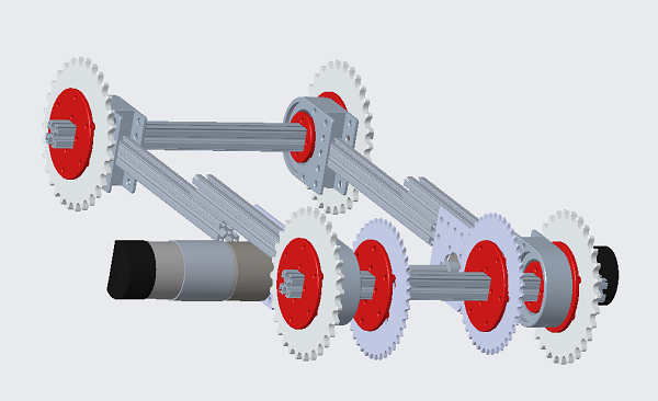
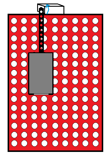
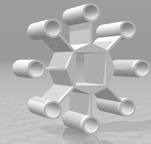
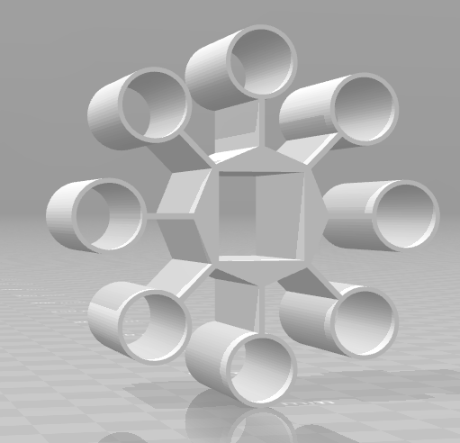
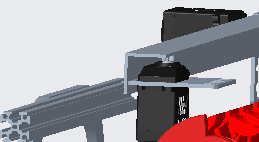
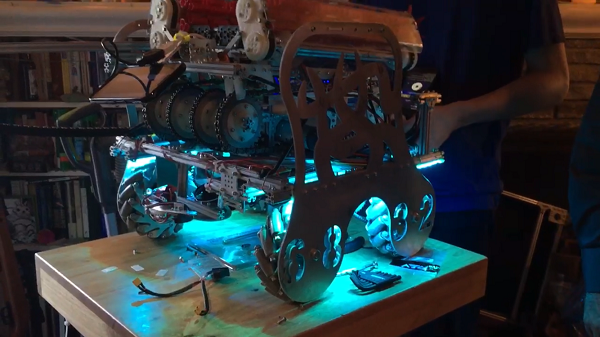
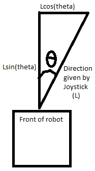
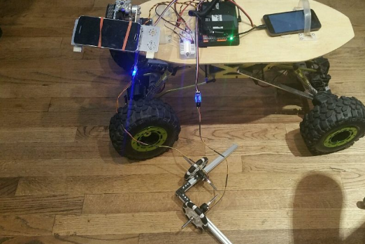
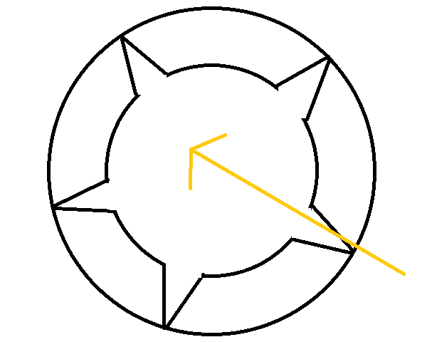
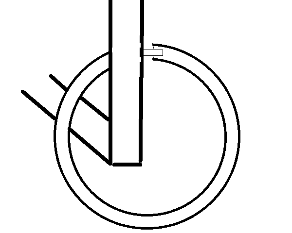
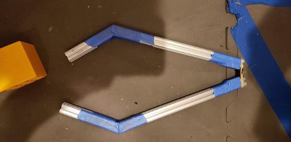
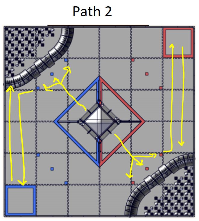
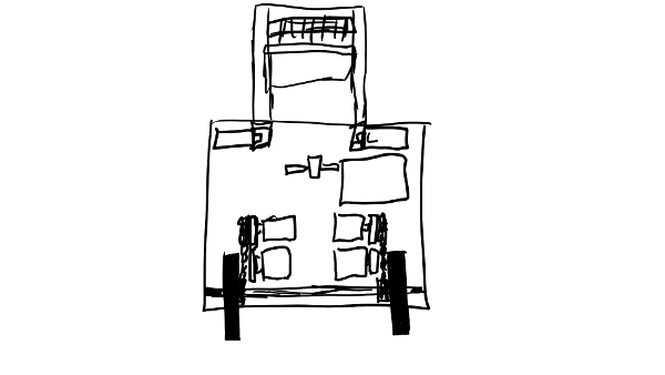
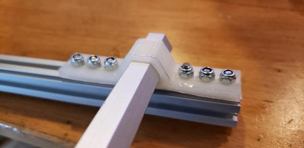
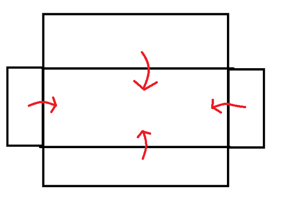
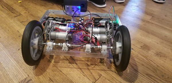
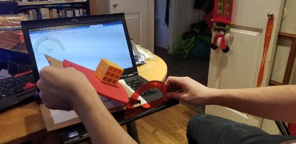
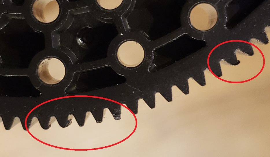
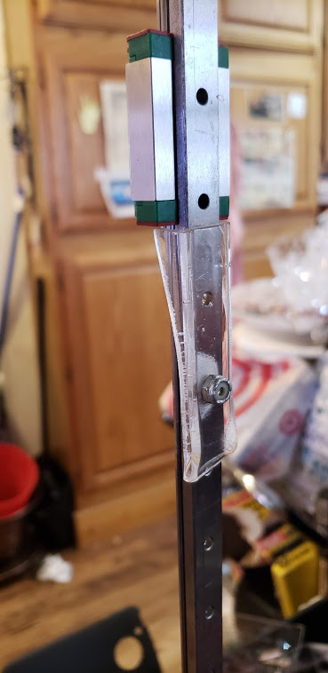
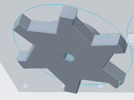
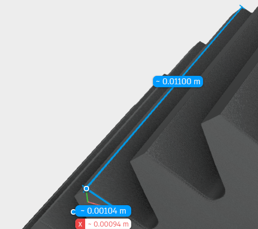
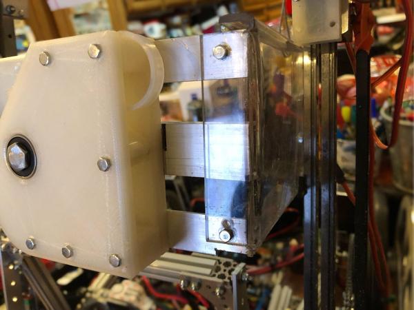
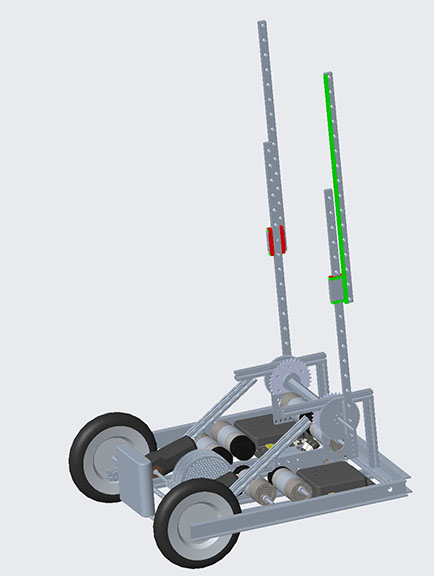
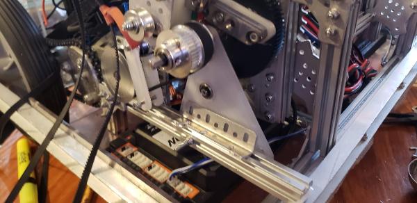
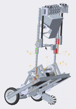
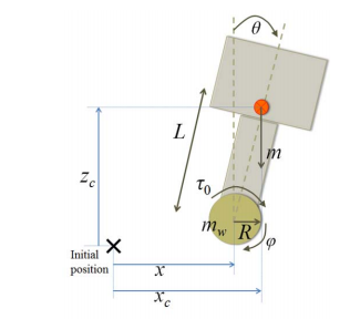
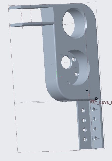
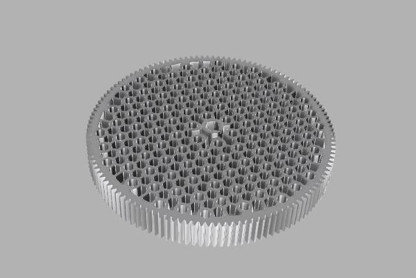
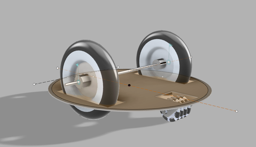
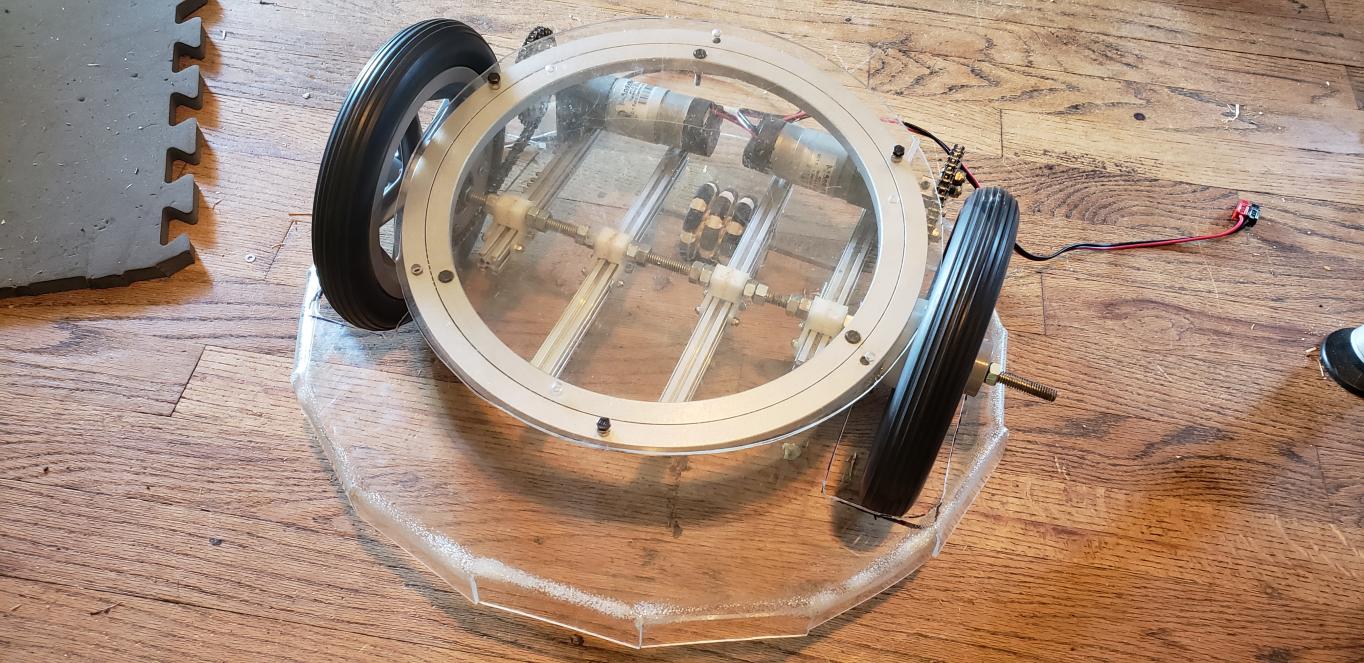
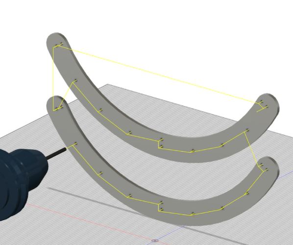
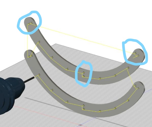
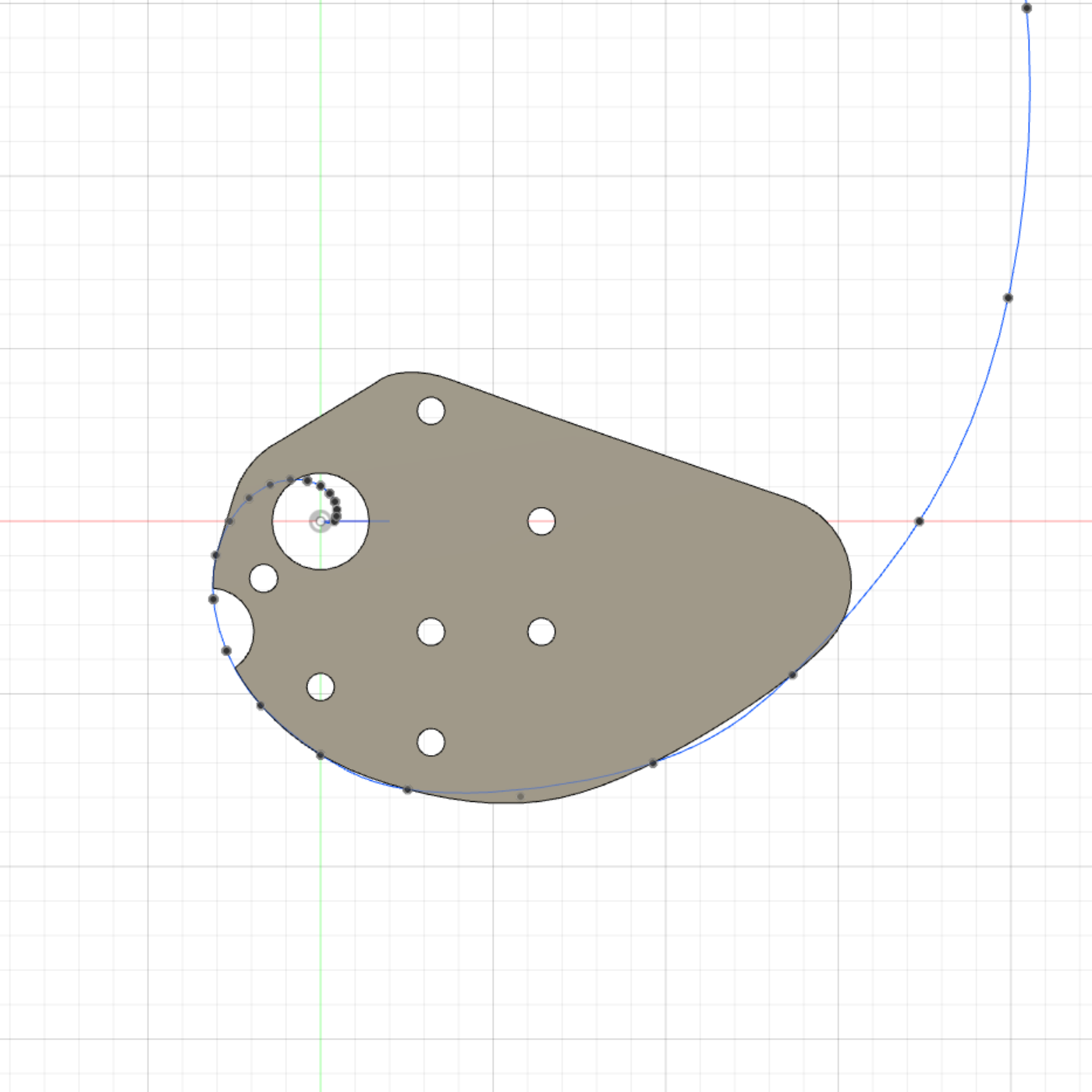
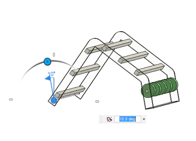
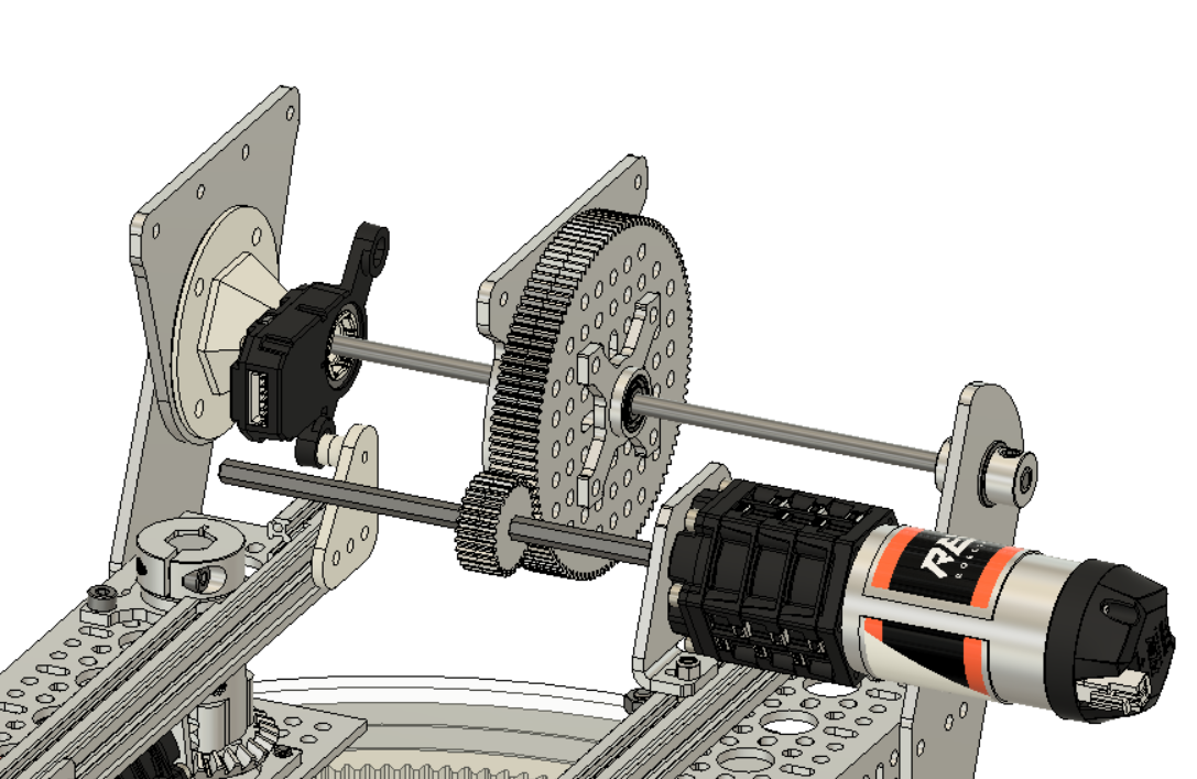
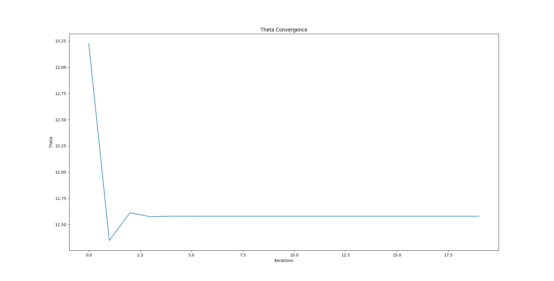
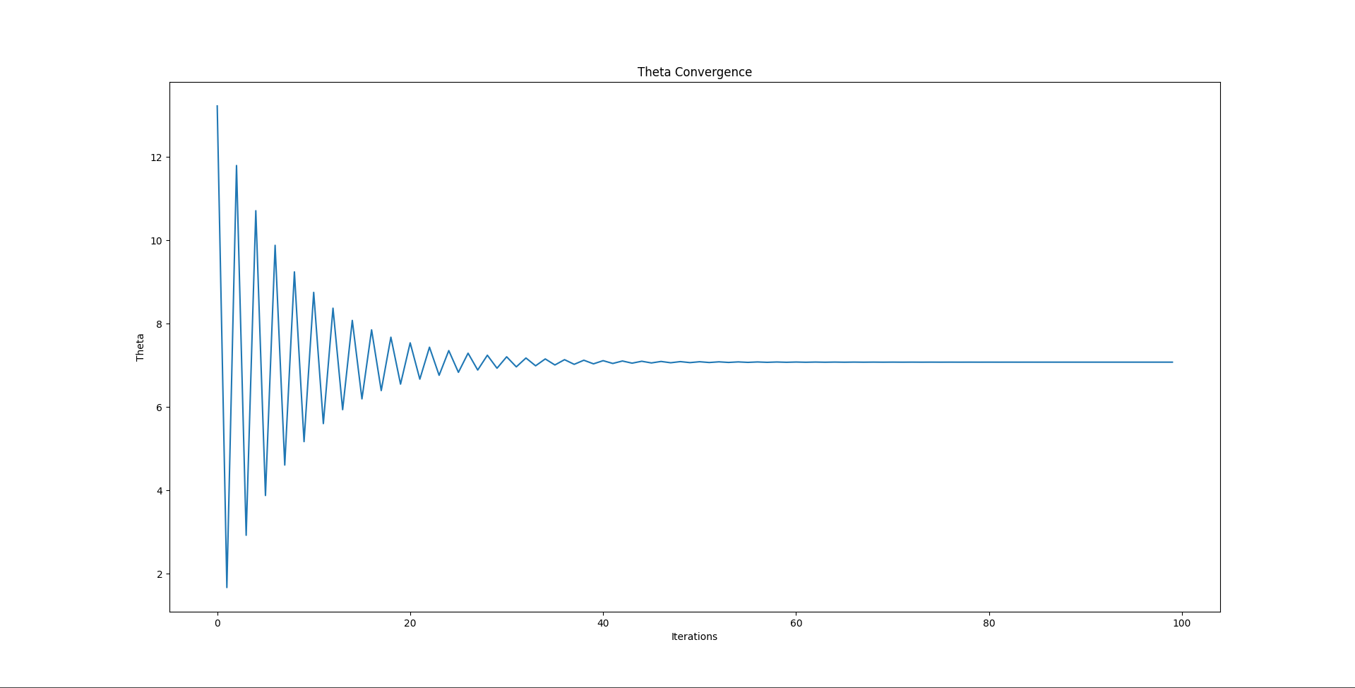
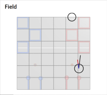
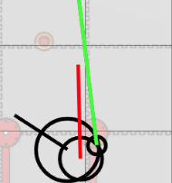
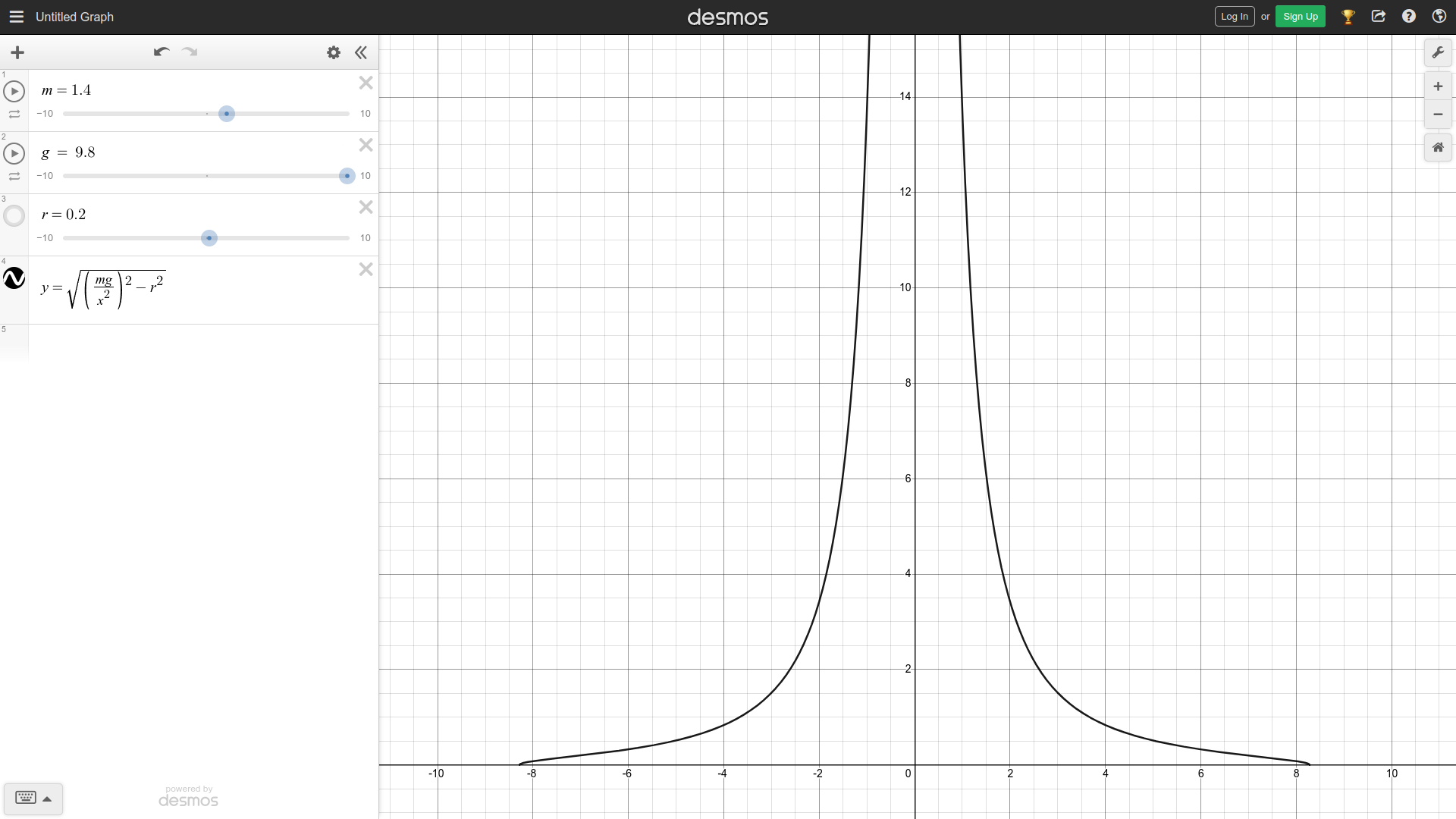
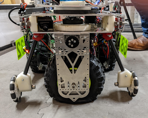
1.1
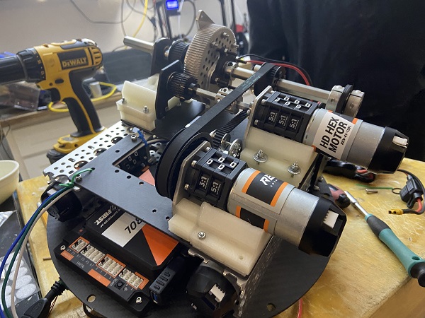
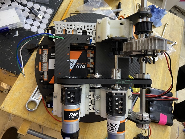
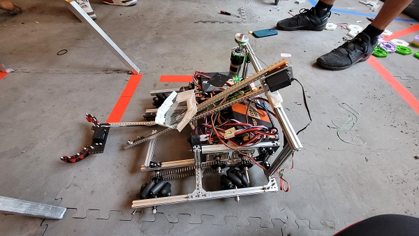
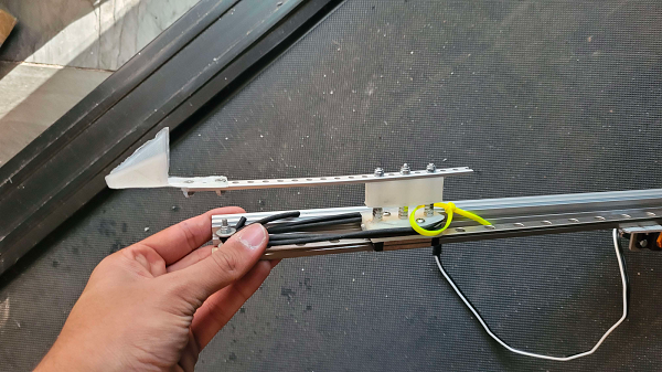
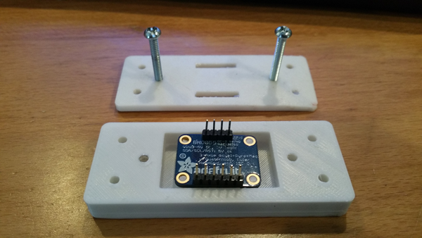
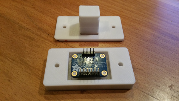
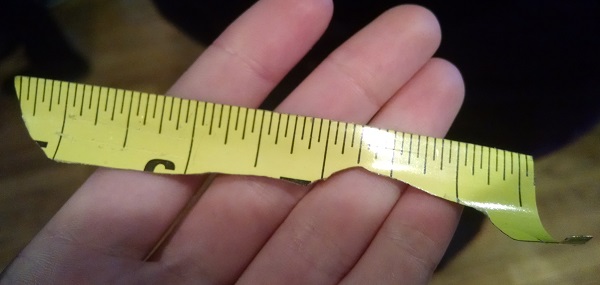
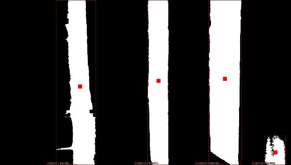
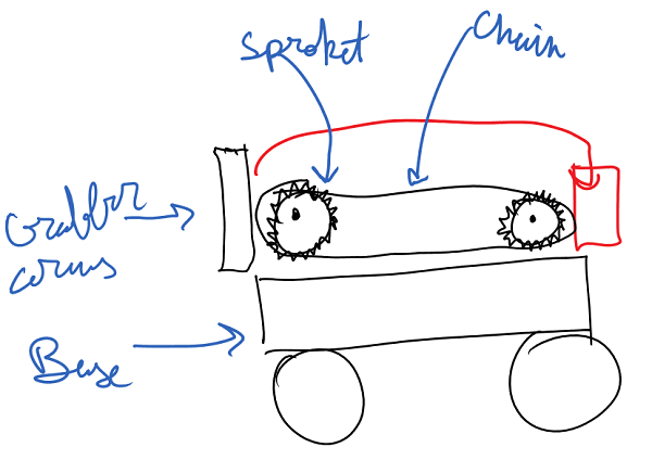
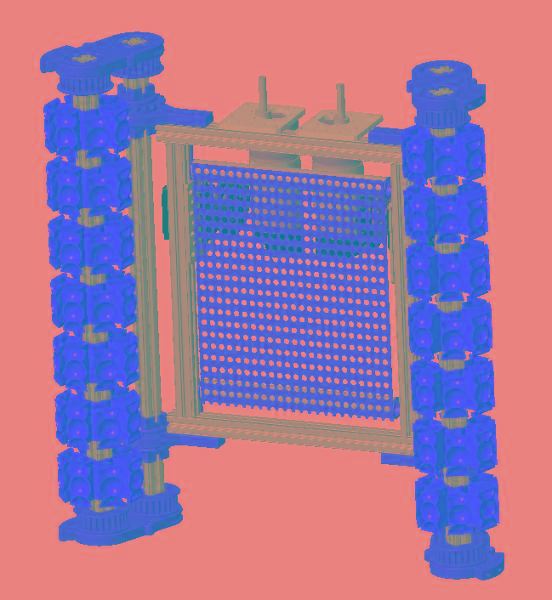
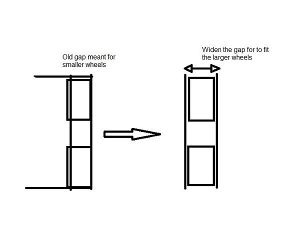
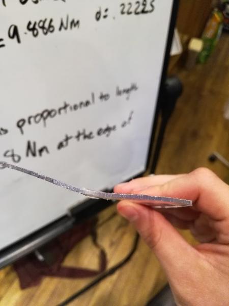
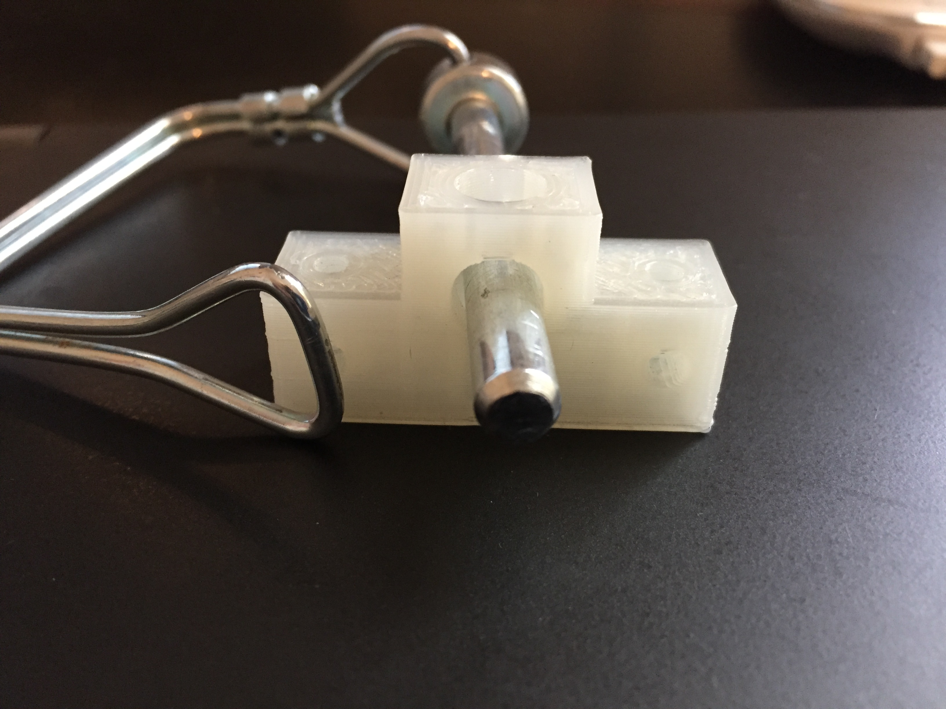
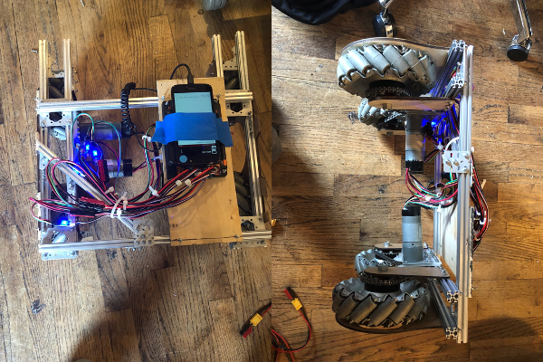
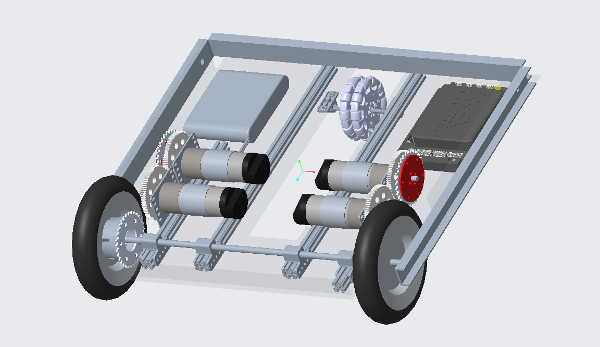
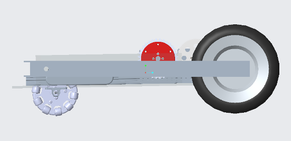
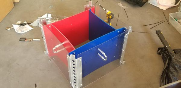
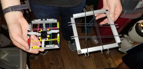
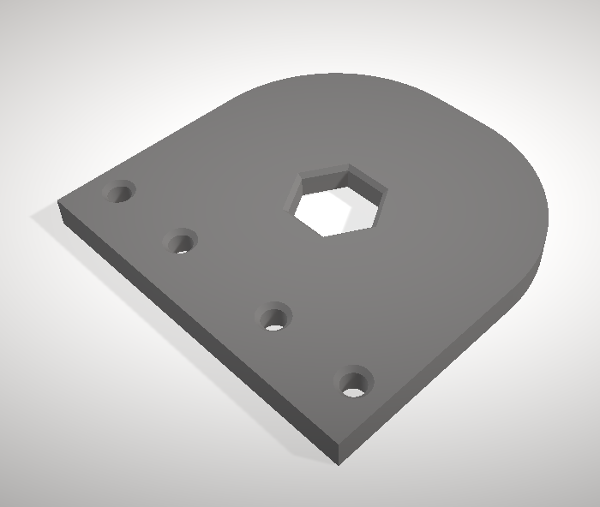
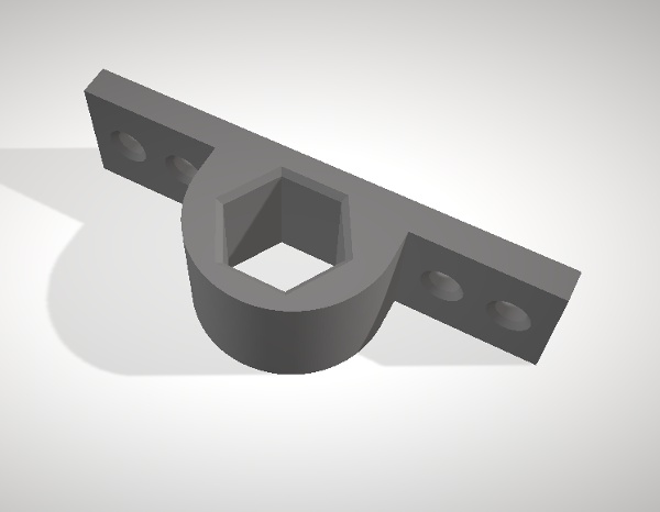
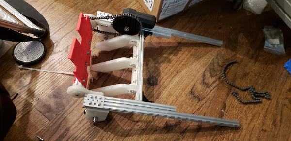
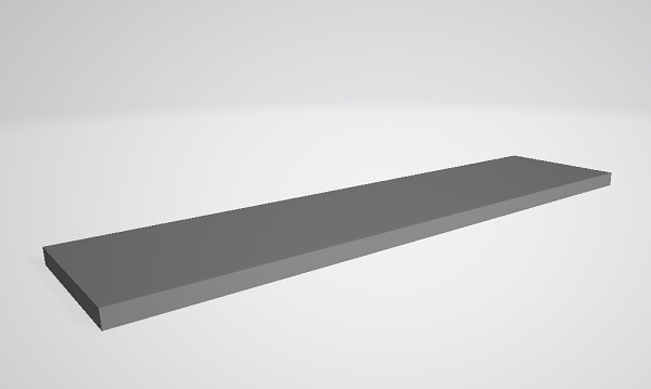
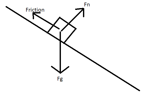
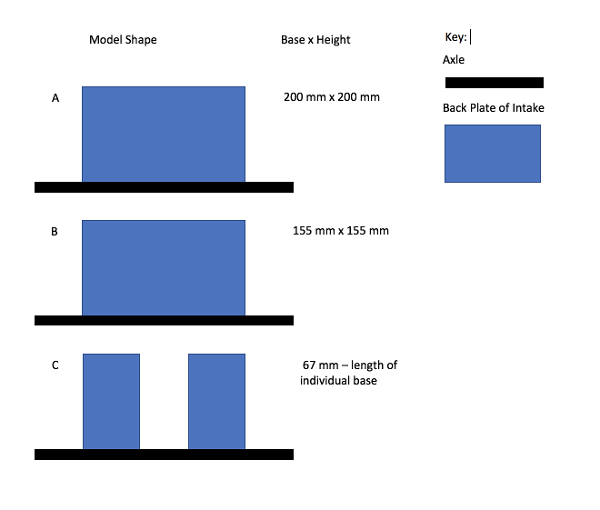
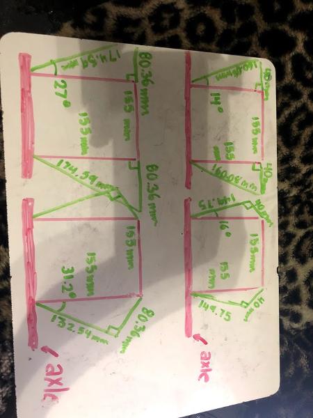
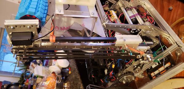
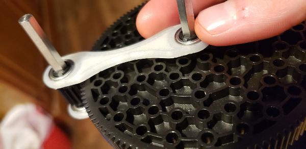
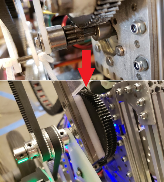
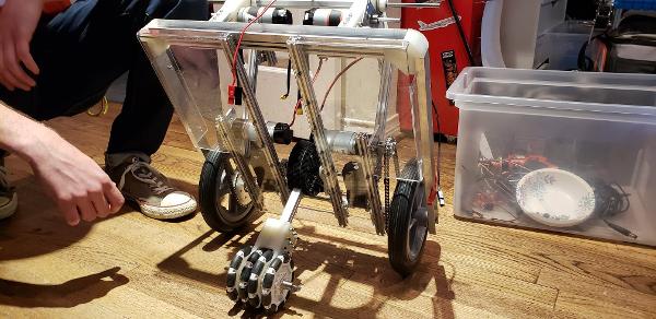
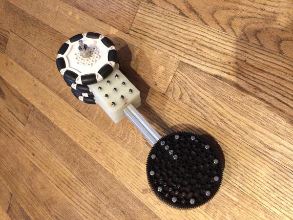
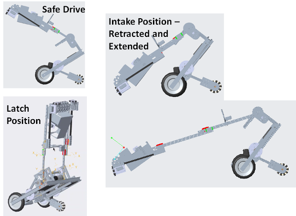
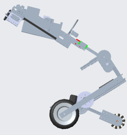
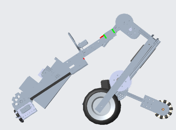
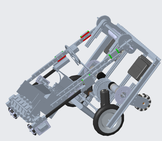
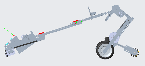
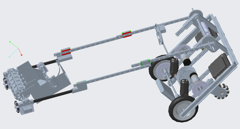
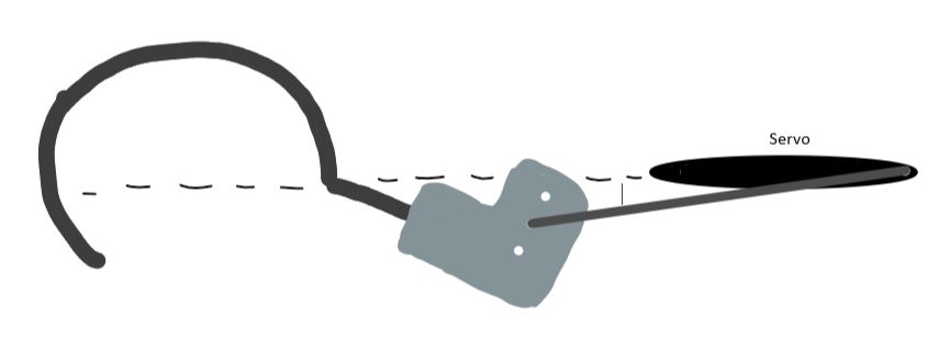
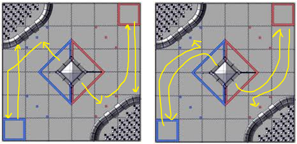
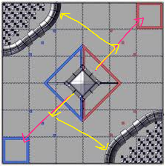
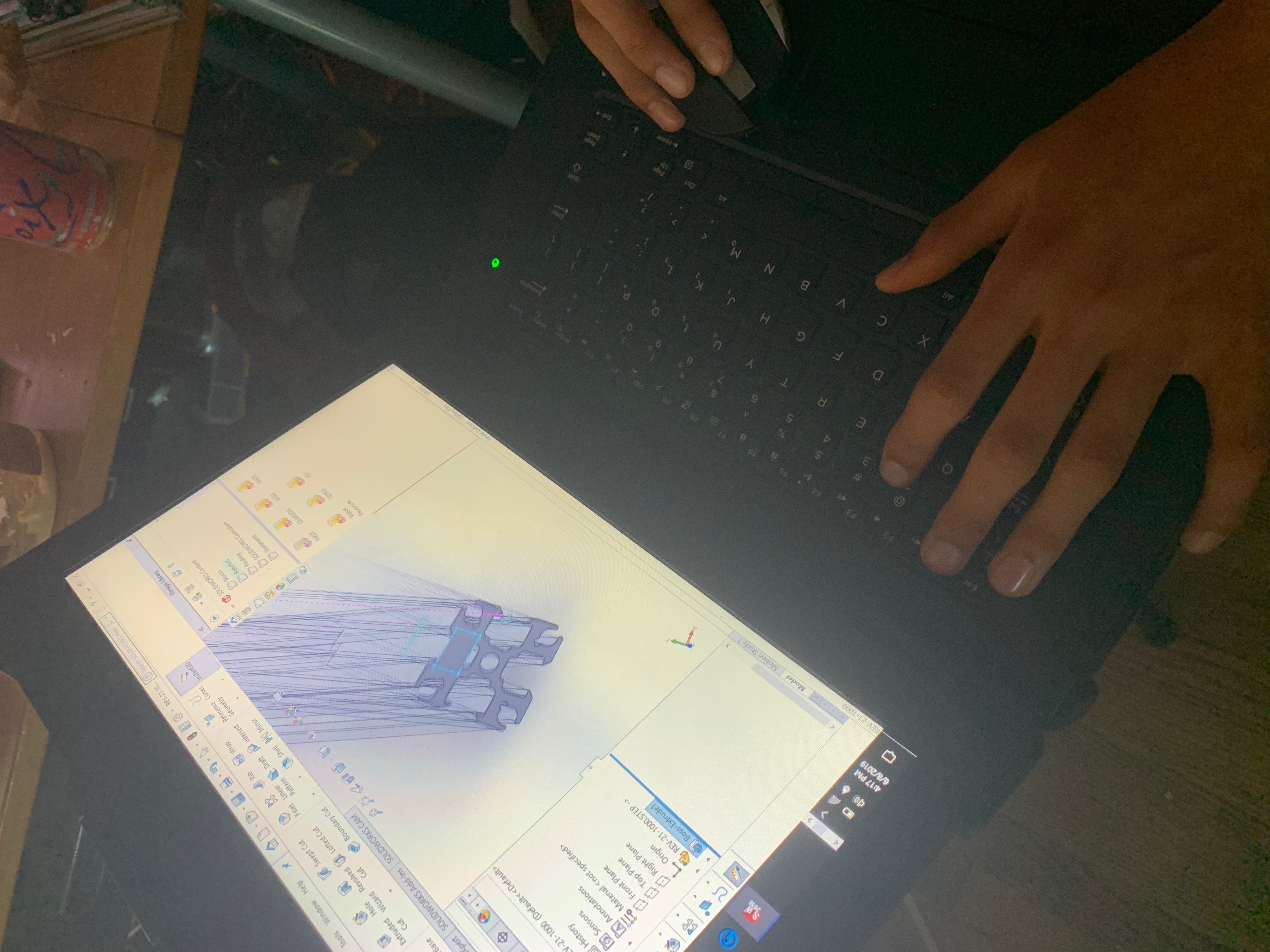
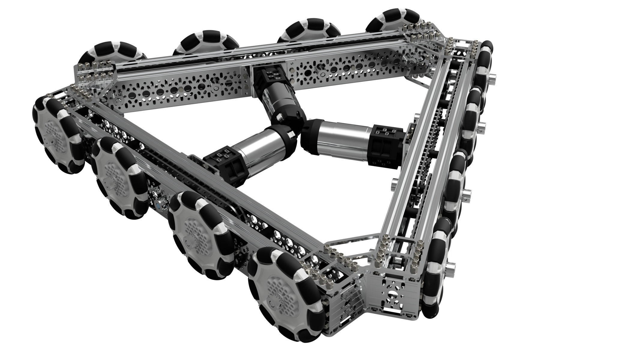
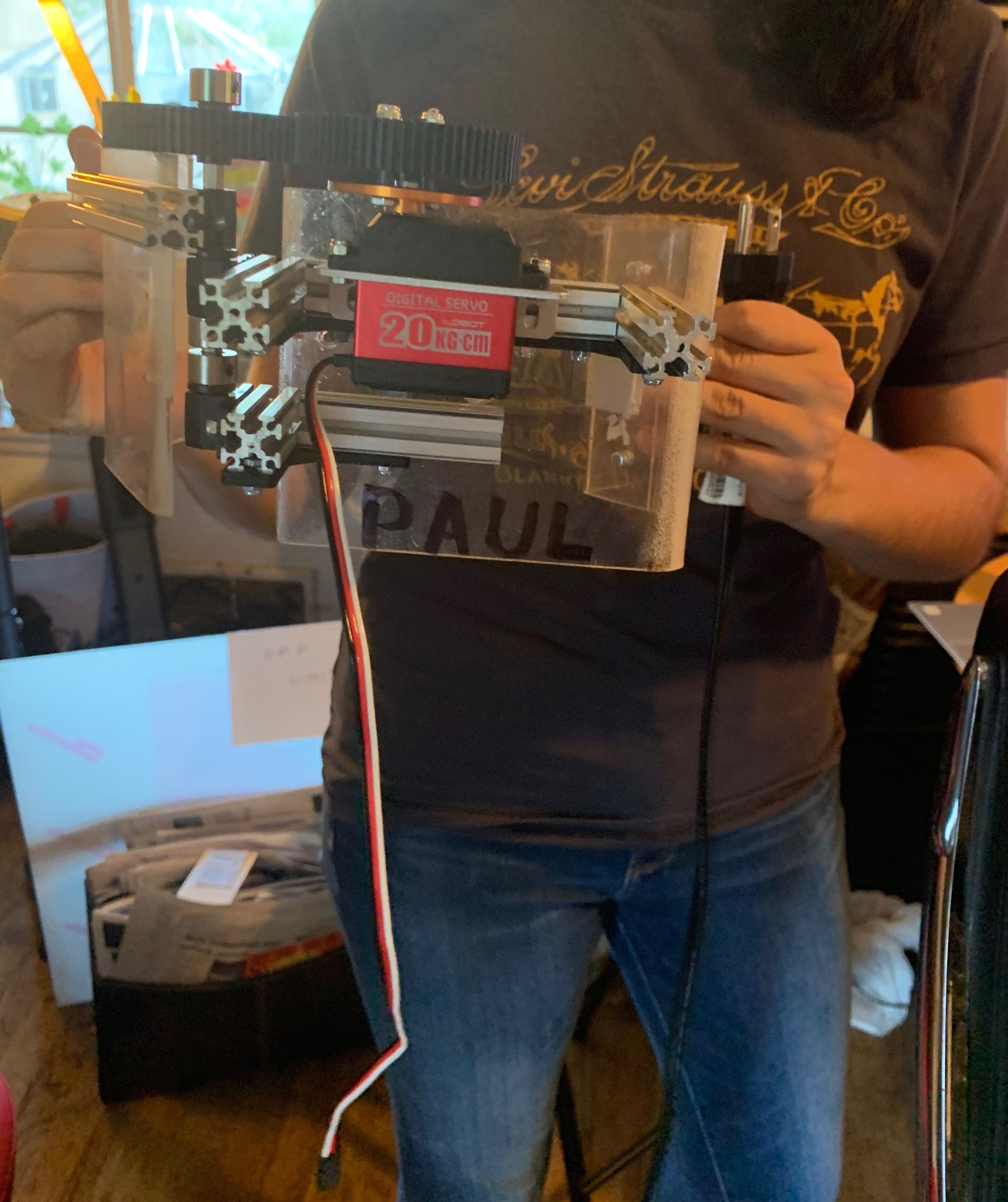
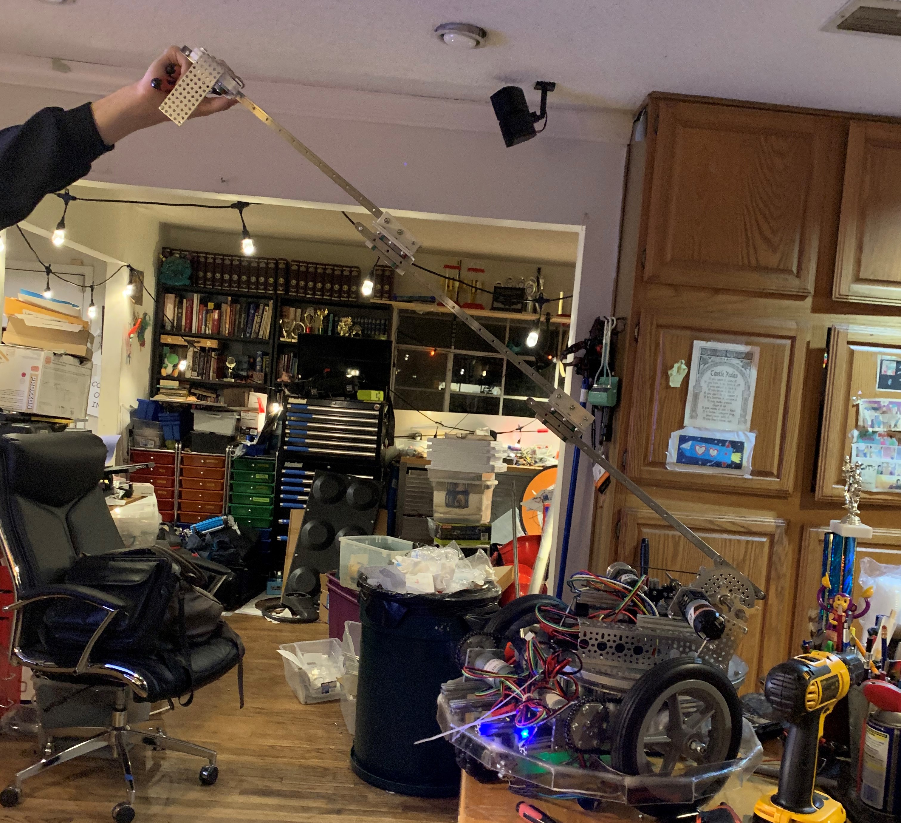
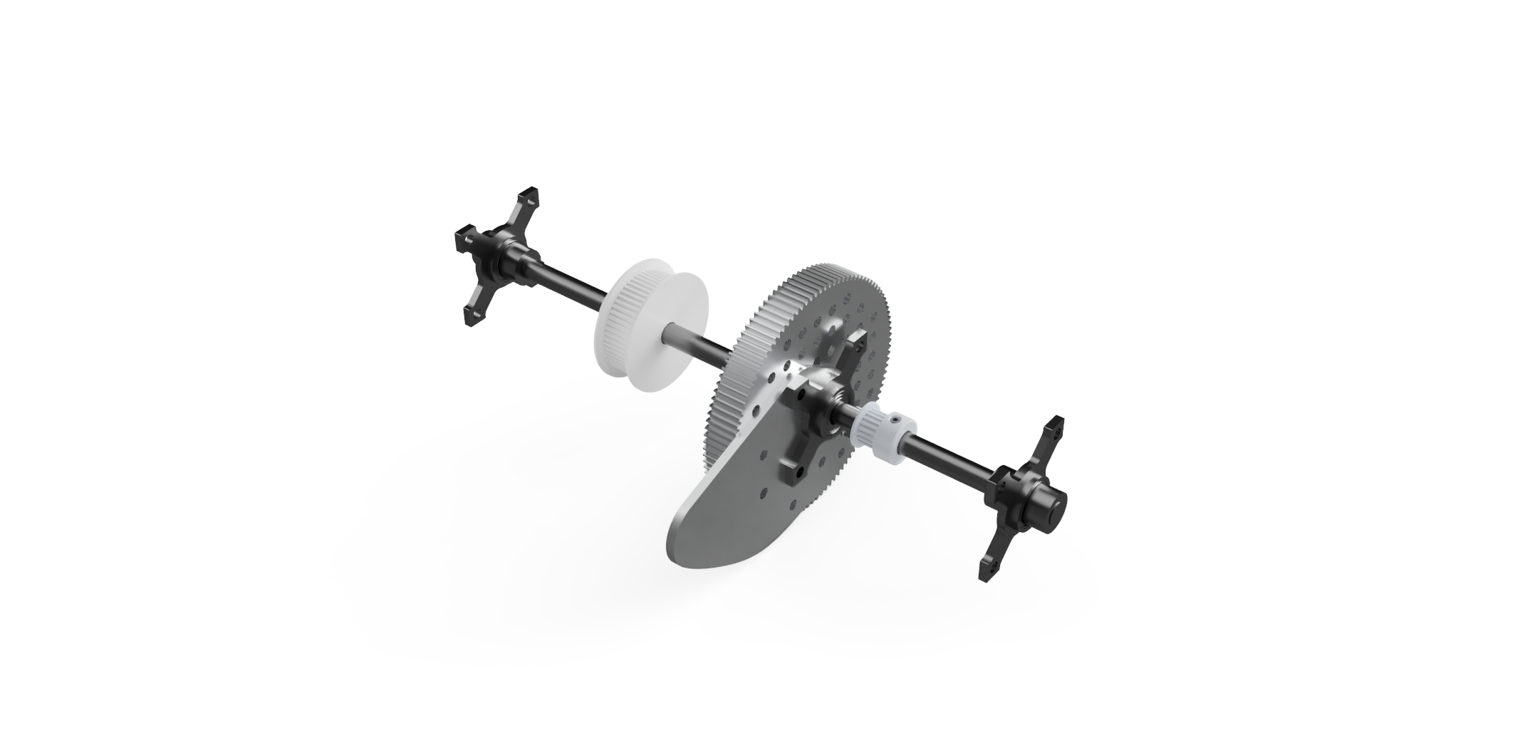
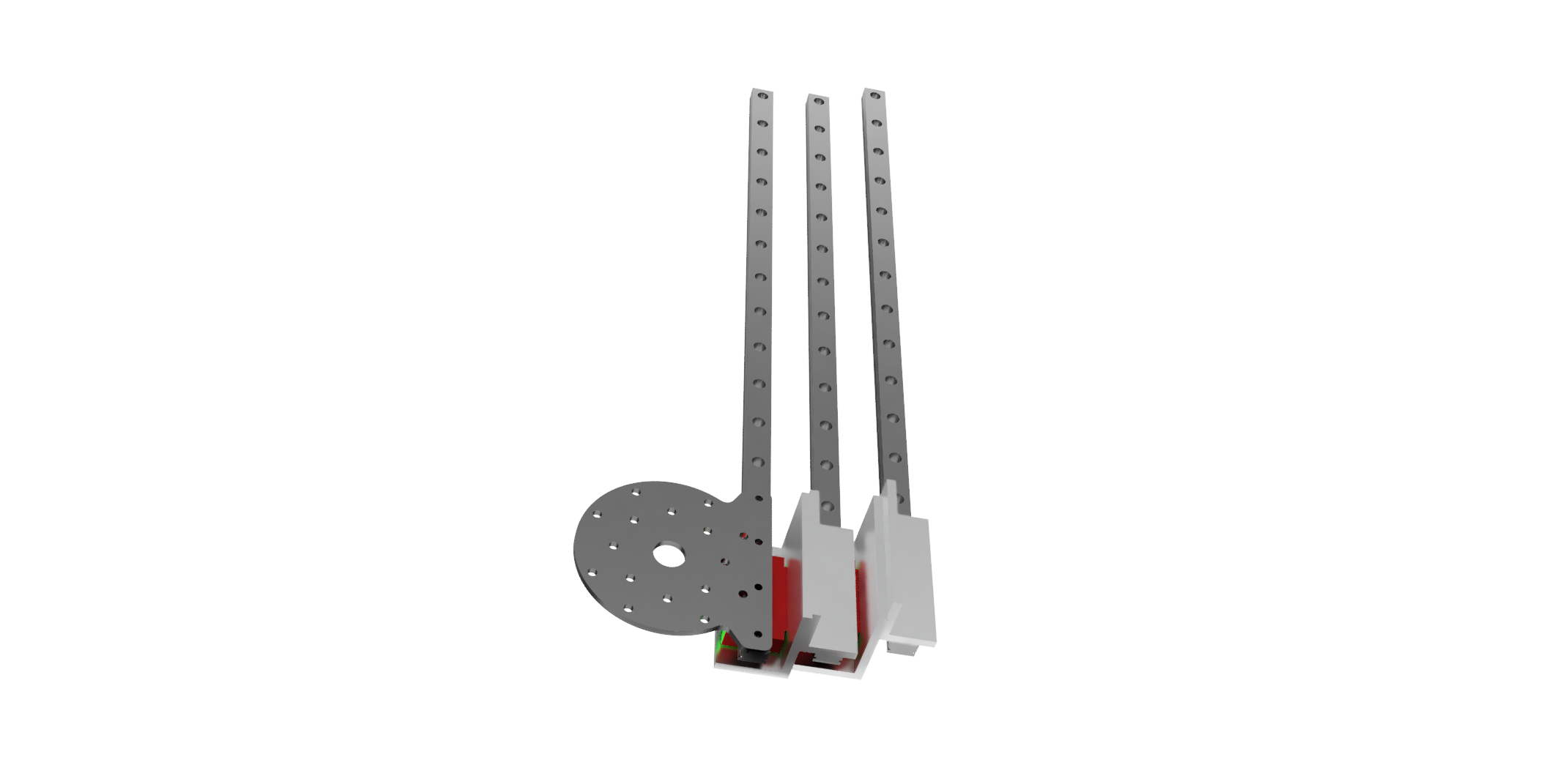
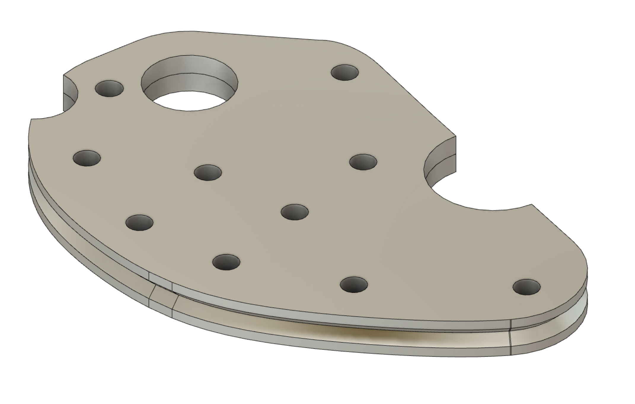
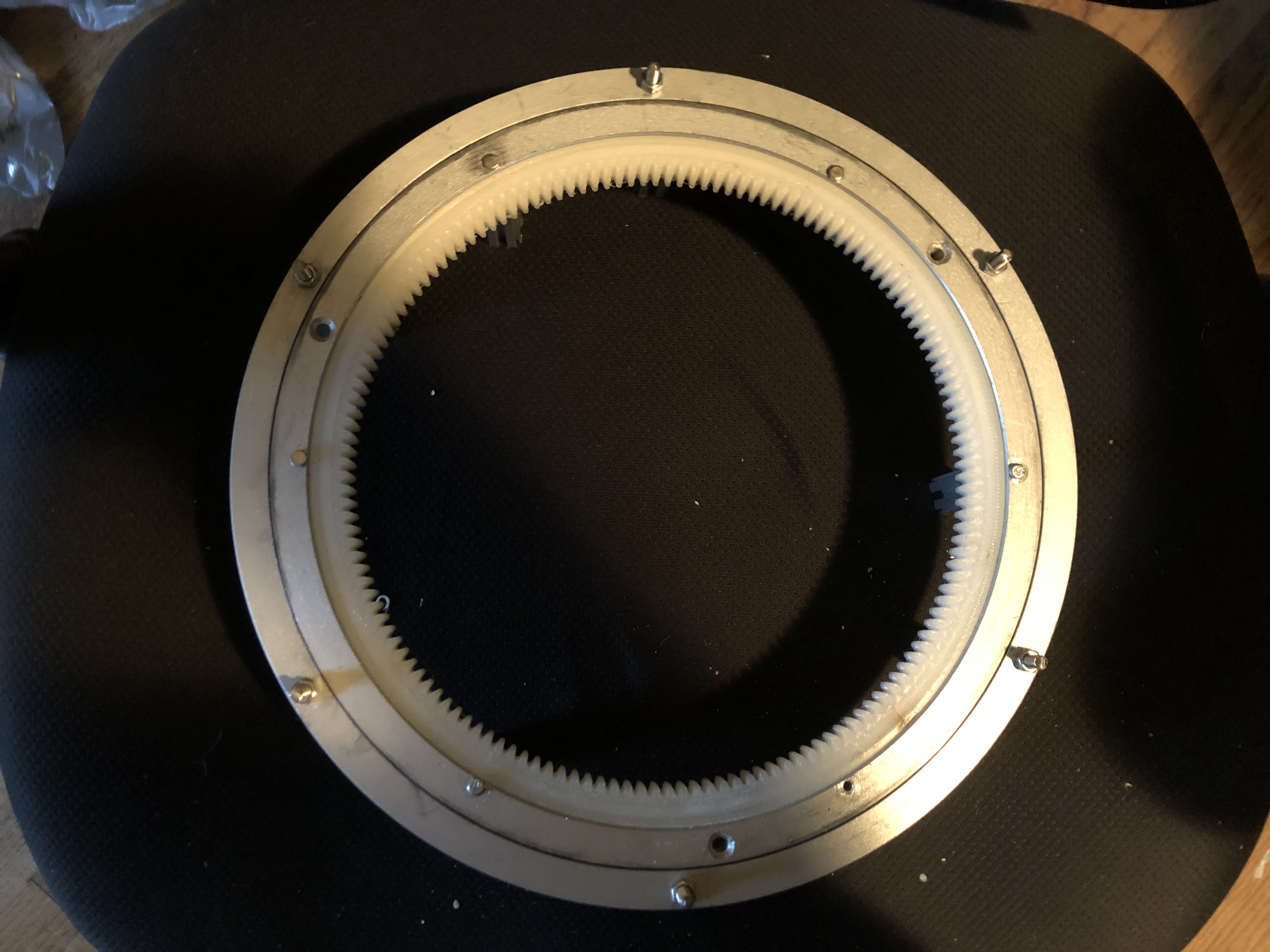
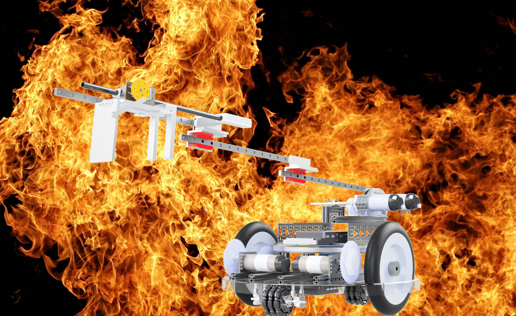
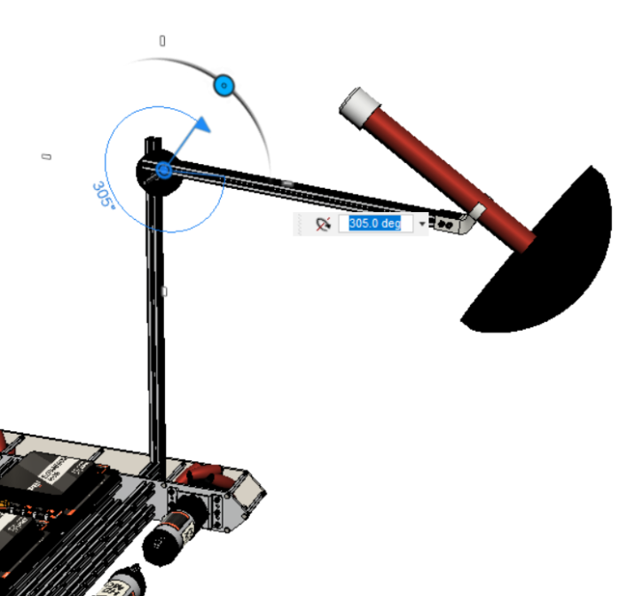
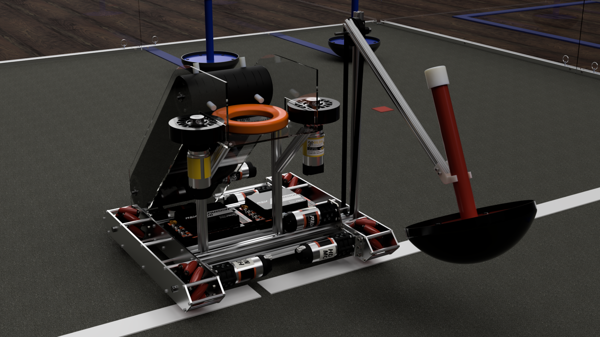
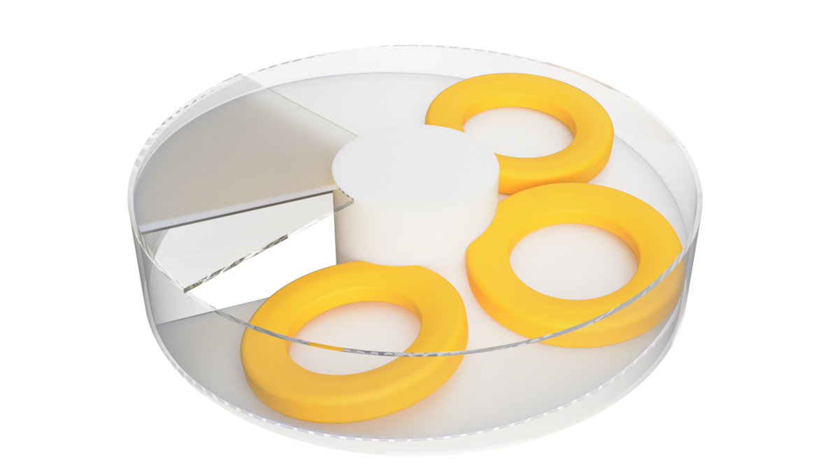
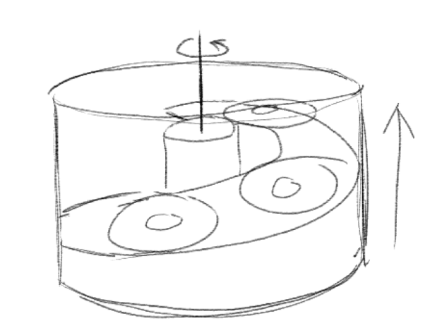
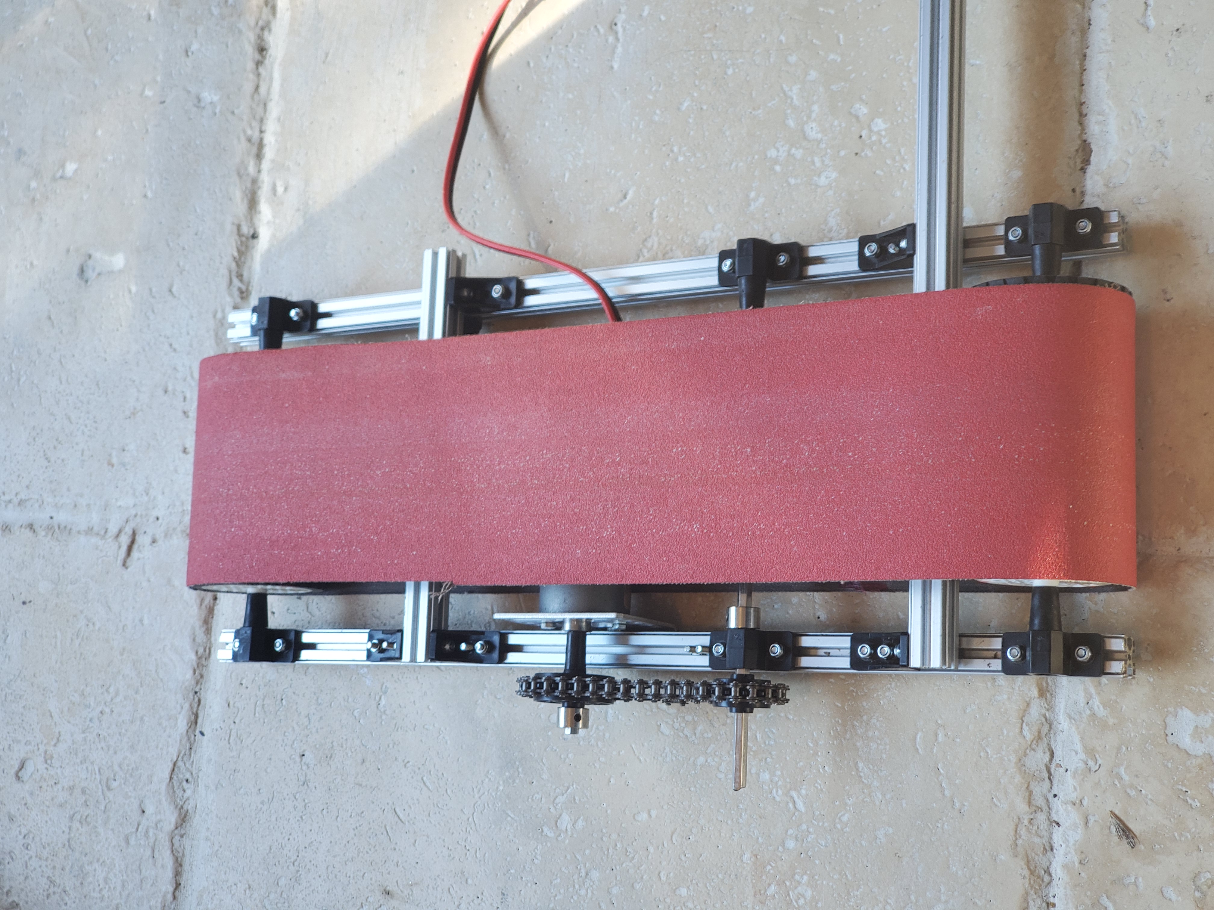
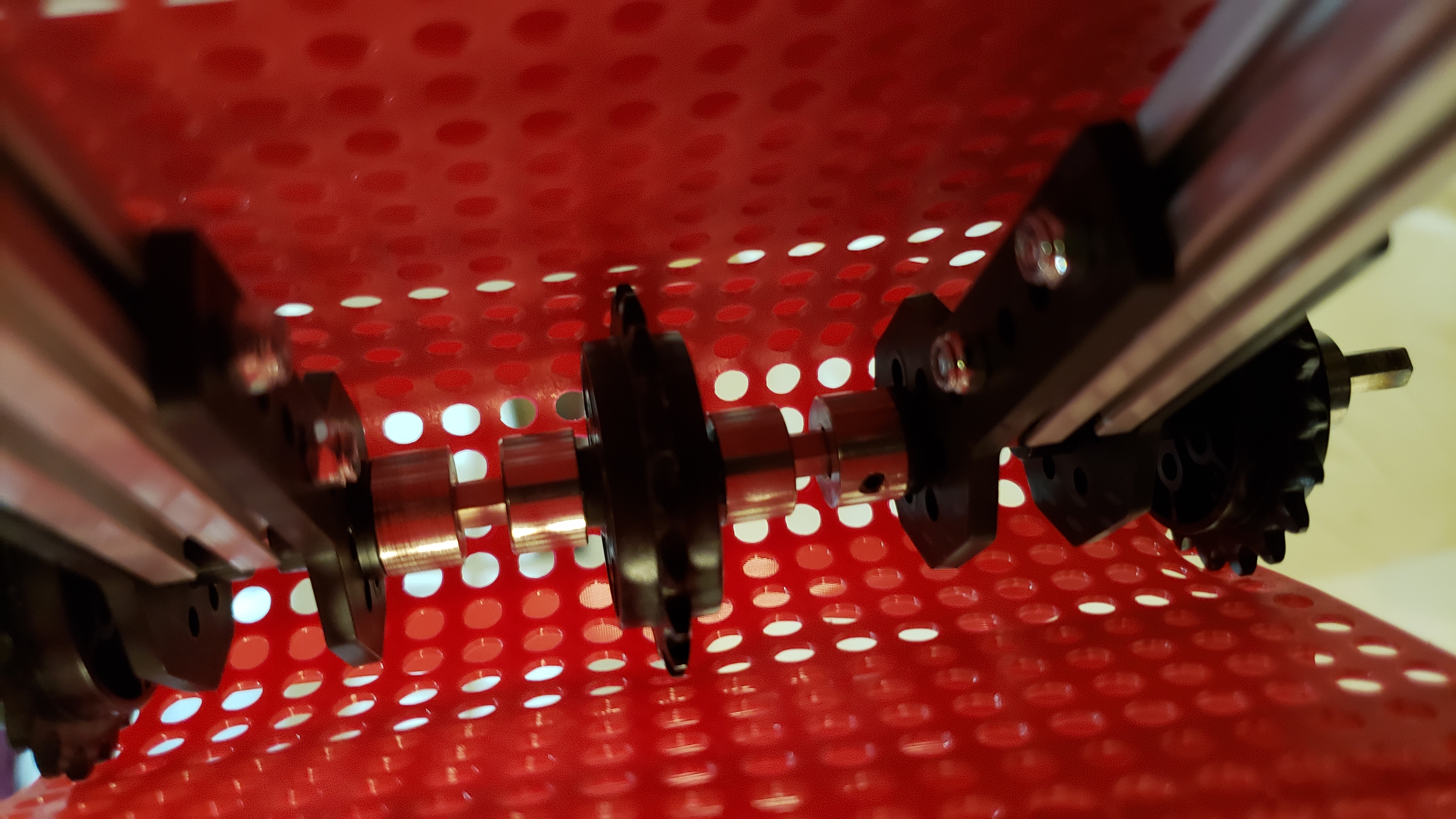
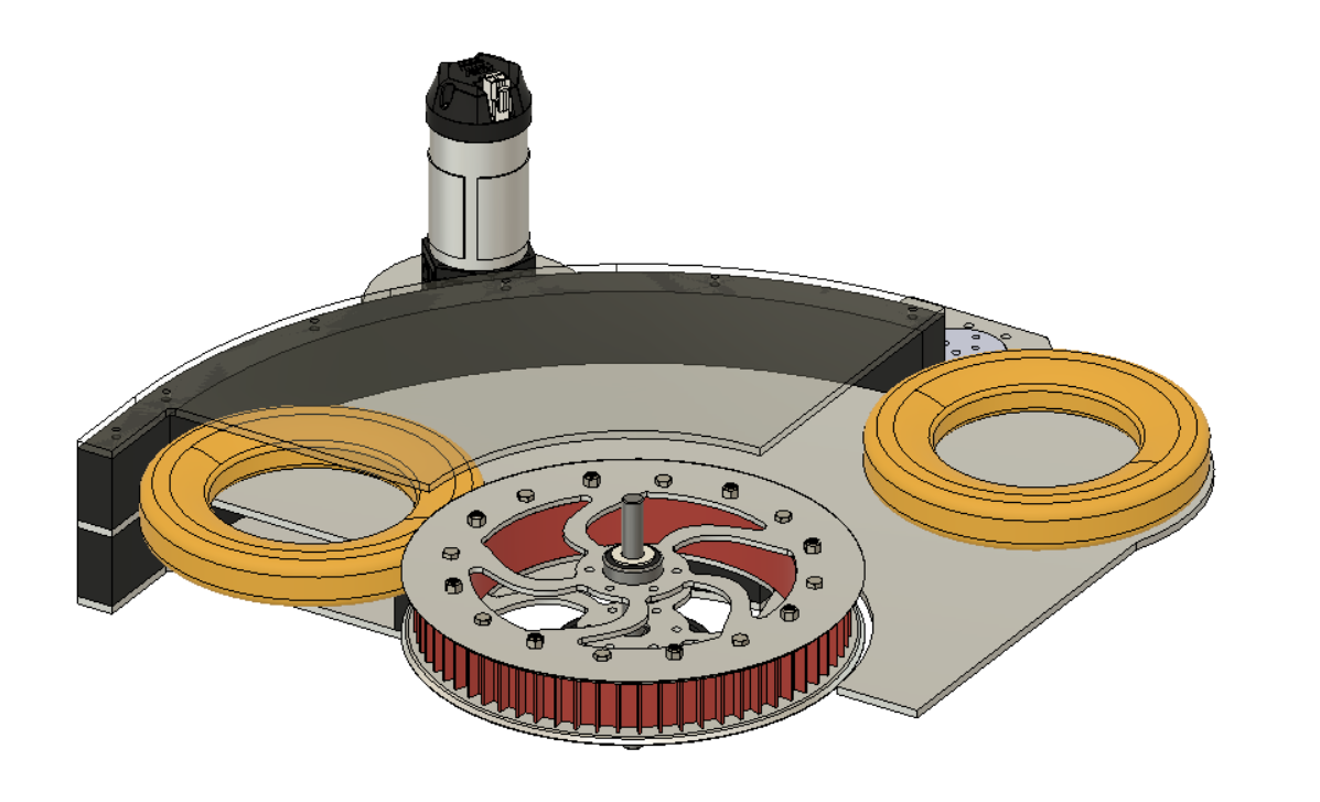
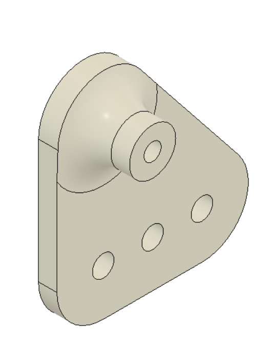
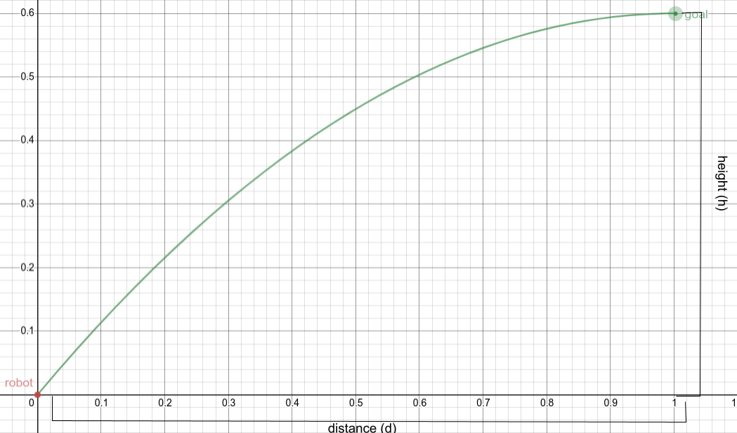
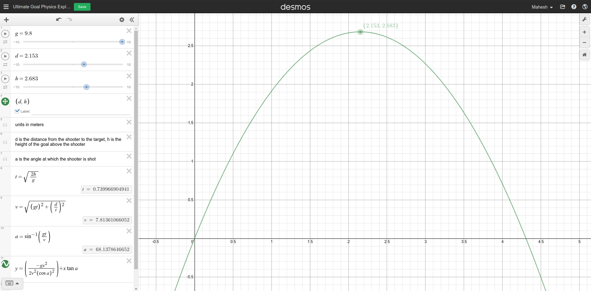
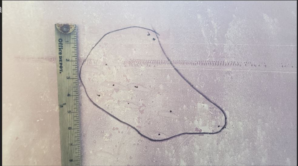
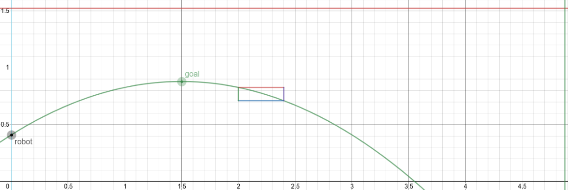
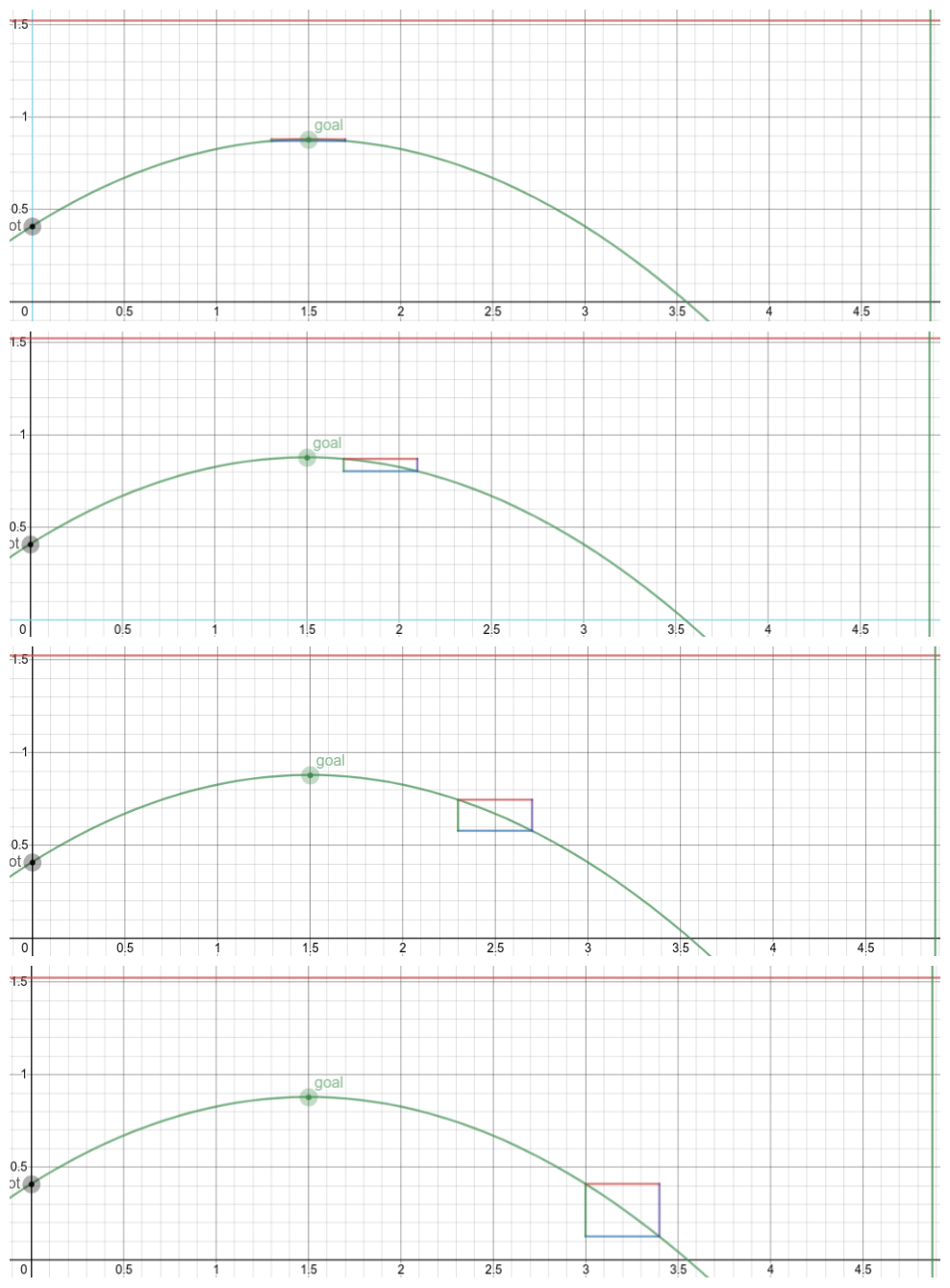
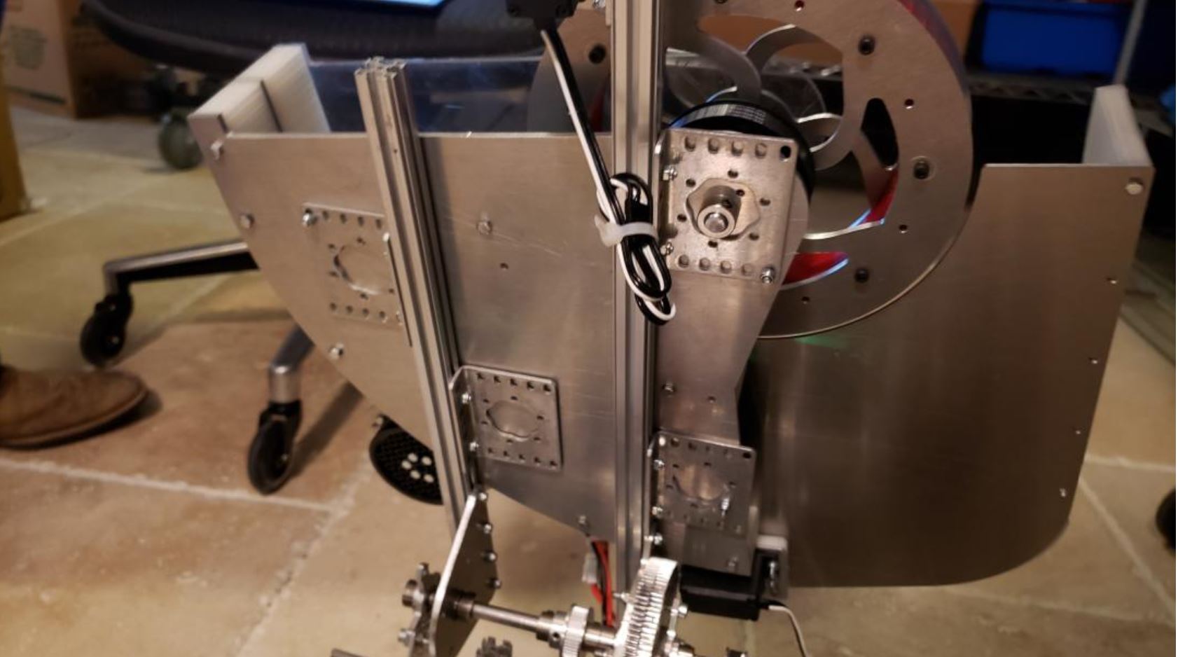
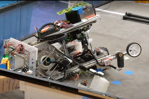
Based on the constants defined and geometry defined in the image below:
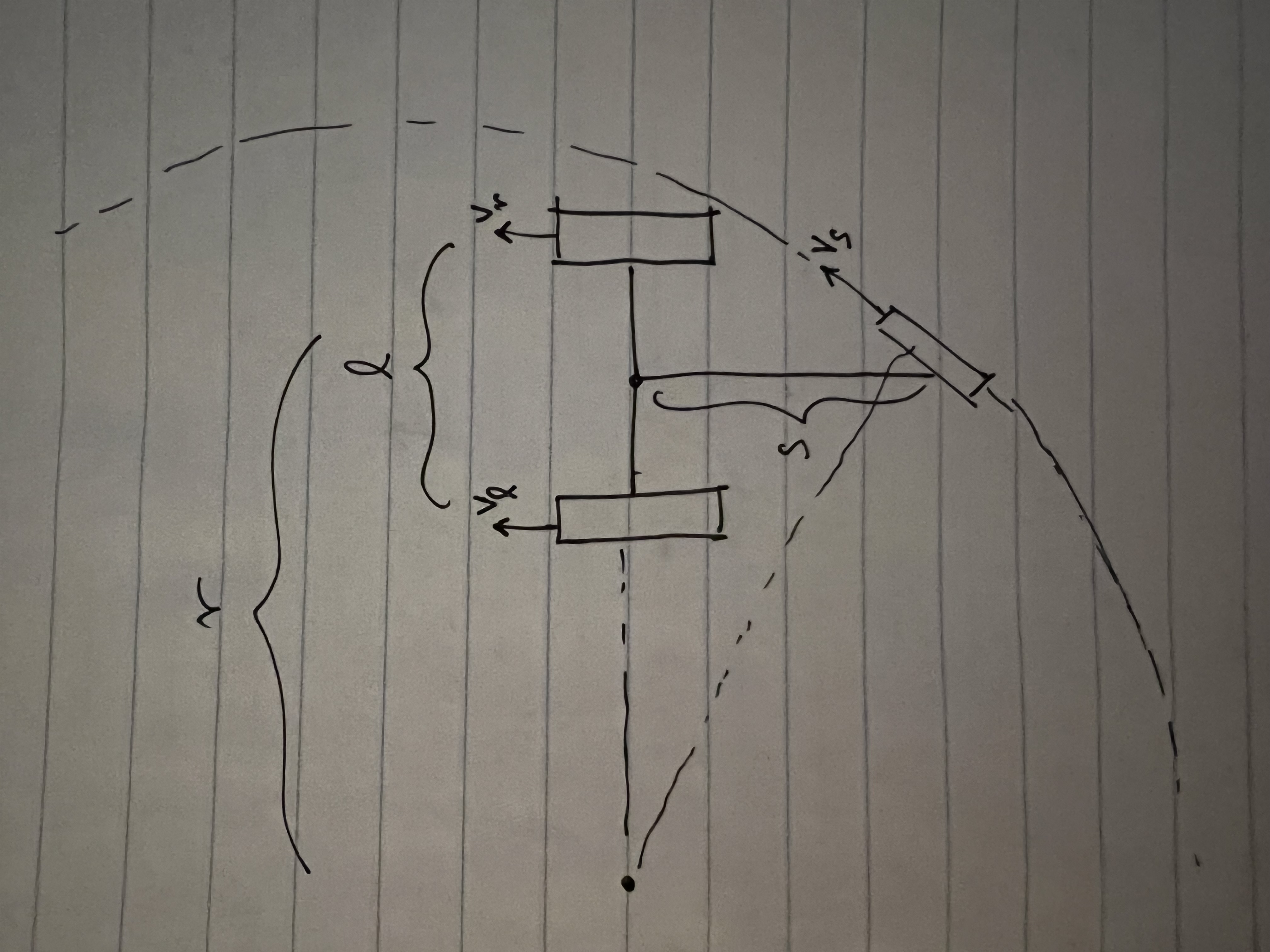
The equation can be applied to the left wheel to derive its inverse
kinematics:
\[\displaylines{\vec{v_l} = \vec{v} + \vec{\omega} \times \vec{r_l} \\ =
\mathbf{v + \omega (r - \frac{l}{2})}}\]
where \(r\) is the turn radius and \(l\) is the width of the robot's front
axle. Applied to the right wheel, the equation yields:
\[\displaylines{\vec{v_r} = \vec{v} + \vec{\omega} \times \vec{r_r} \\ =
\mathbf{v + \omega (r + \frac{l}{2})}}\]
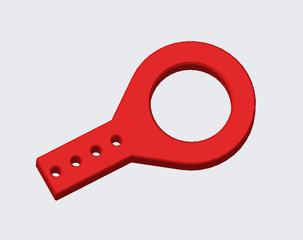
Applied to the swerve wheel, the equation yields:
\[\displaylines{\vec{v_s} = \vec{v} + \vec{\omega} \times \vec{r_s} \\ =
\mathbf{v + \omega \sqrt{r^2 + s^2}}}\]
where \(s\) is the length of the chassis (the distance between the front
axle and swerve wheel).
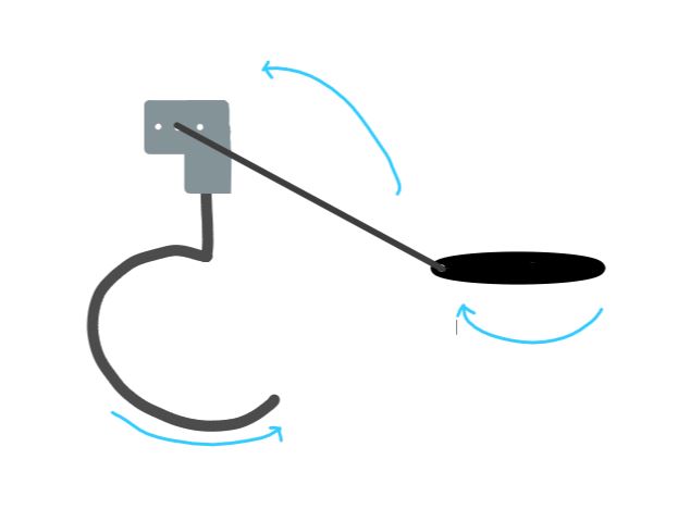
The angle of the swerve wheel can then be calculated like so using the
geometry of the robot:
\[\displaylines{\theta = \frac{\pi}{2} - tan^{-1}\left( \frac{s}{r}
\right)}\]
Mathematically/intuitively, the equations check out as well. When only
rotating (\(v = 0\)), \(r = \frac{v}{\omega} = \frac{0}{\omega} = 0\), so:
\[\displaylines{ v_l = v + \omega(r - \frac{l}{2}) = \omega \cdot
-\frac{l}{2} \\ v_r = v + \omega(r + \frac{l}{2}) = \omega \cdot
\frac{l}{2} \\ v_s = v + \omega\sqrt{r^2 + s^2} = \omega \cdot \sqrt{ s^2}
= \omega \cdot s}\]
In all three cases, \(v = \omega \cdot r\), where \(r\) is the distance
from each wheel to the "center of the robot", defined as the midpoint of
the front axle. Since rotating without translating will be around a center
of rotation equal to the center of the robot, the previous definition for
\(r\) can be used.
As for the equation for \(\theta\), the angle of the swerve wheel, it
checks out intuitively as well. When only translating (driving straight:
\(\omega = 0\)), \(r = \frac{v}{\omega} = \frac{v}{0} = \infty\), so:
\[\displaylines{ \theta = \frac{\pi}{2} - tan^{-1} \left( \frac{s}{r}
\right) \\ = \frac{\pi}{2} - tan^{-1} \left( \frac{s}{\infty} \right) \\ =
\frac{\pi}{2} - tan^{-1}(0) \\ = \frac{\pi}{2} - 0 \\ = \frac{\pi}{2} }\]
As expected, when translating, \(\theta = 0\), as the swerve wheel must
point straight for the robot to drive straight. When only rotating (\(v =
0\)), \(r = \frac{v}{\omega} = \frac{0}{\omega} = 0\), so:
\[\displaylines{ \theta = \frac{\pi}{2} - tan^{-1} \left( \frac{s}{r}
\right) \\ = \frac{\pi}{2} - tan^{-1} \left( \frac{s}{0} \right) \\ =
\frac{\pi}{2} - tan^{-1}(\infty) \\ = \frac{\pi}{2} - \lim_{x \to +\infty}
tan^{-1}(x) \\ = \frac{\pi}{2} - \frac{\pi}{2} \\ = 0}\]
As expected, when only translating (driving straight), \(\theta =
\frac{\pi}{2}\), or in other words, the swerve wheel is pointed directly
forwards to drive the robot directly forwards. When only rotating,
\(\theta = 0\), or in other words, the swerve wheel is pointed directly to
the right to allow the robot to rotate counterclockwise.
Next Steps:
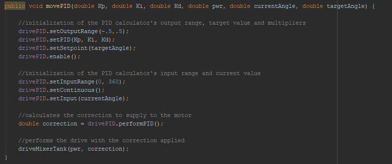
The next step is to use PID control to maintain target velocities and
angles calculated using the derived inverse kinematic equations. Then,
these equations can be used in future motion planning/path planning
attempts to get the robot to follow a particular desired \(v\) and \(
\omega\).
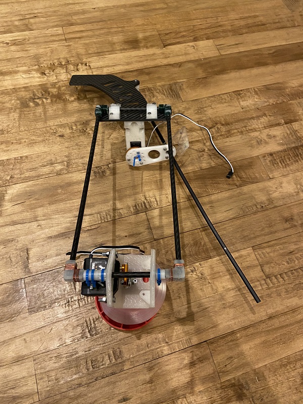
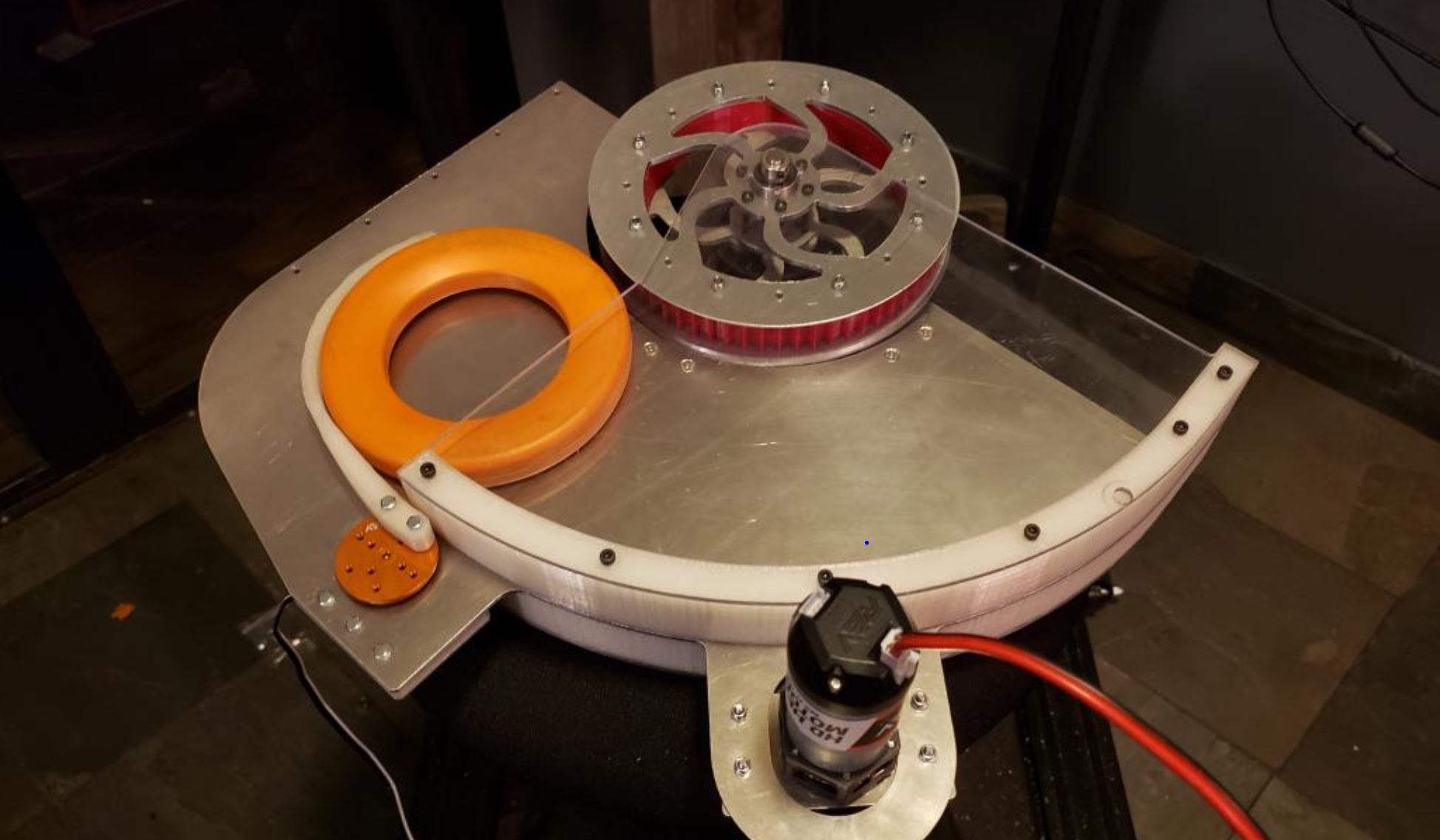
A distance sensor will also need to be used to calculate \(s\), the
distance between the front axle and swerve wheel of the robot.
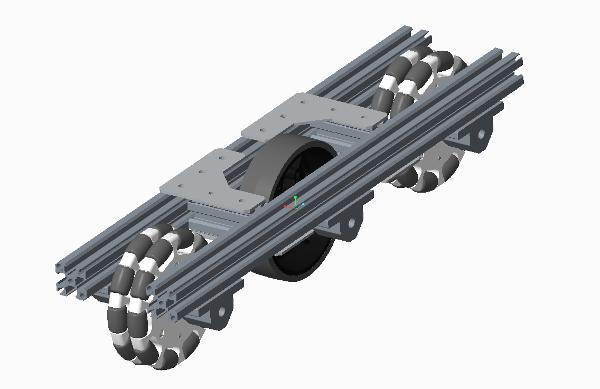
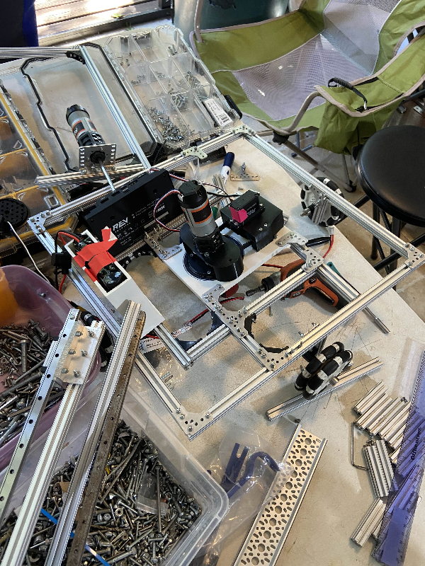
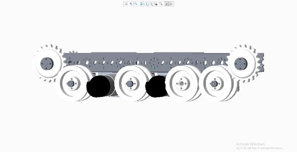
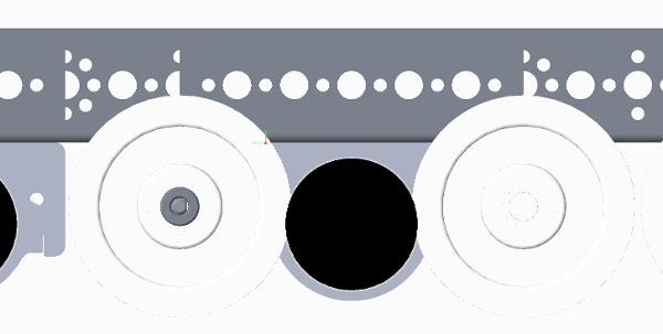
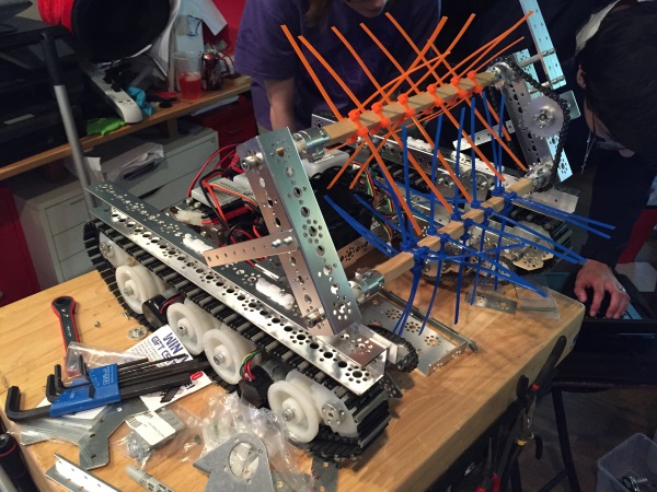
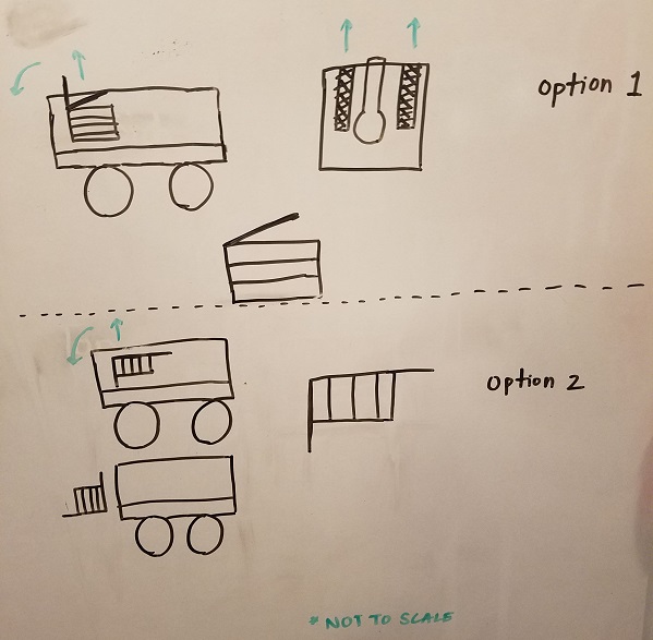
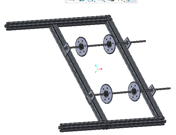
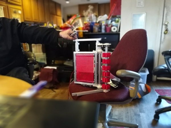
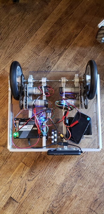
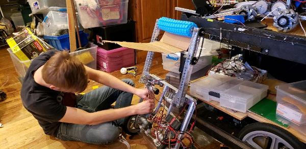
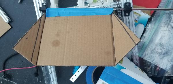
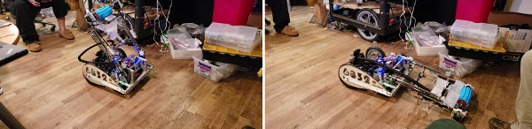
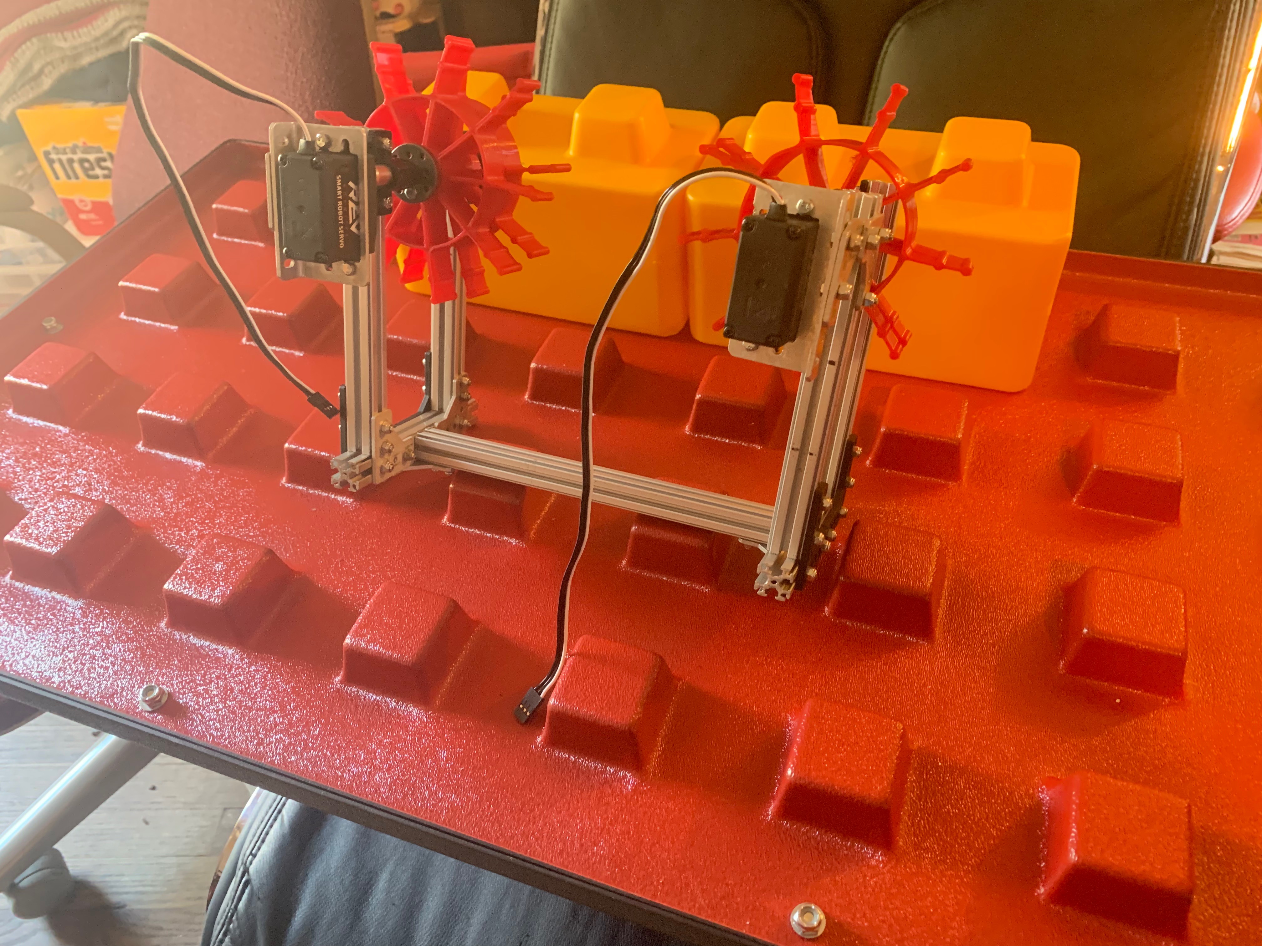
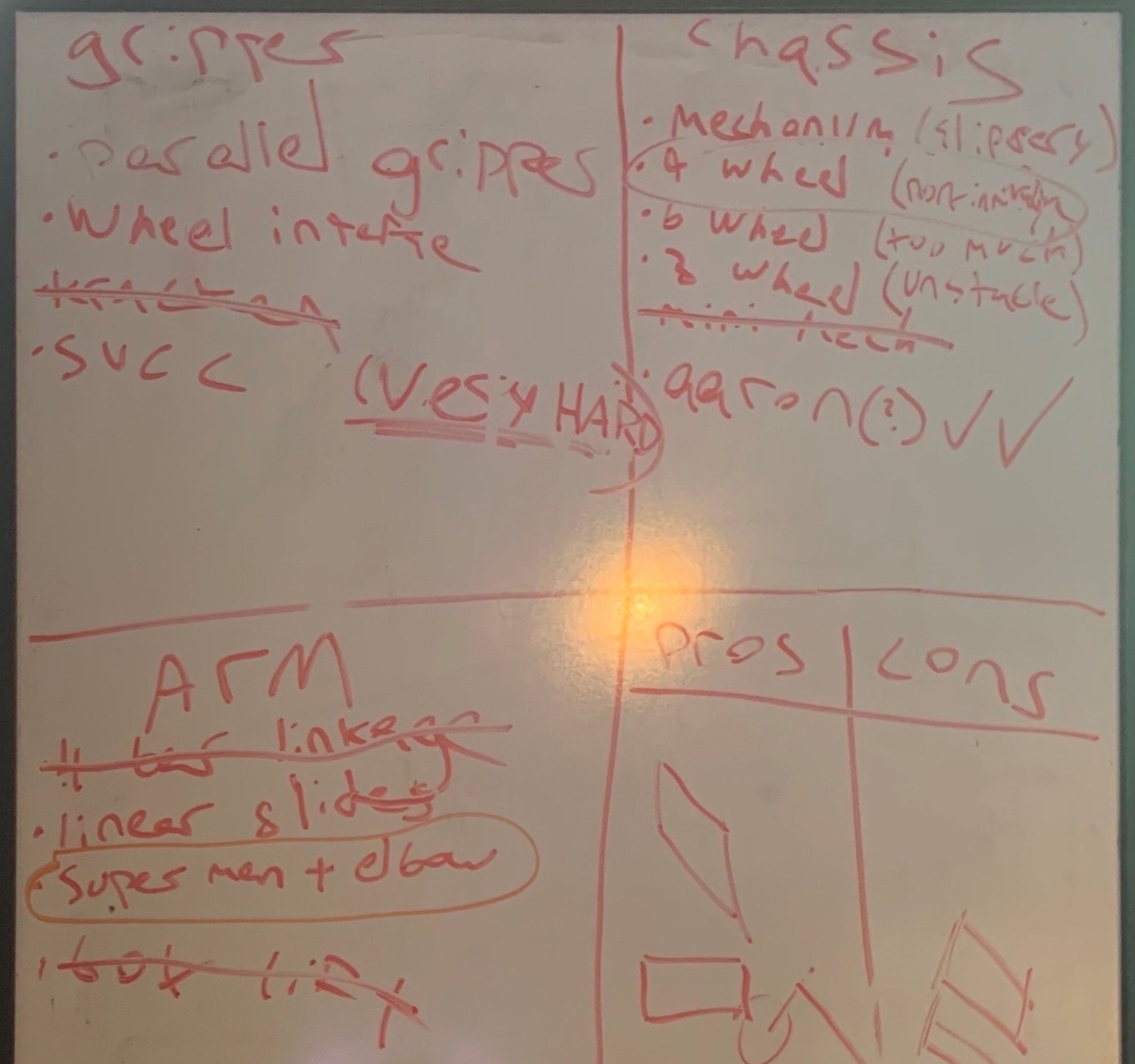
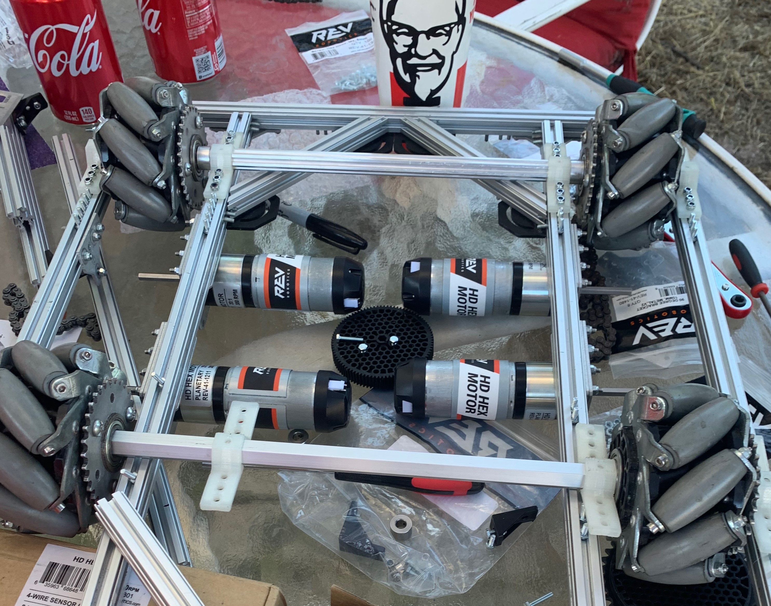
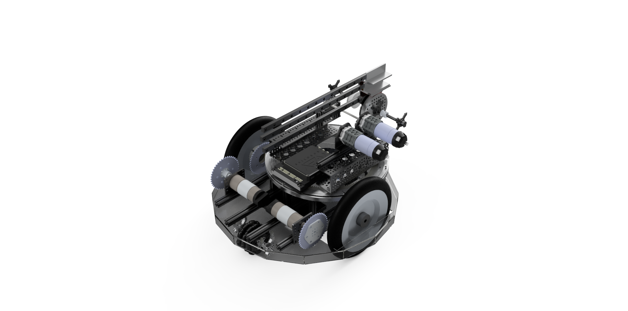
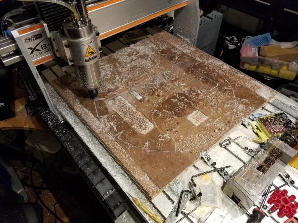
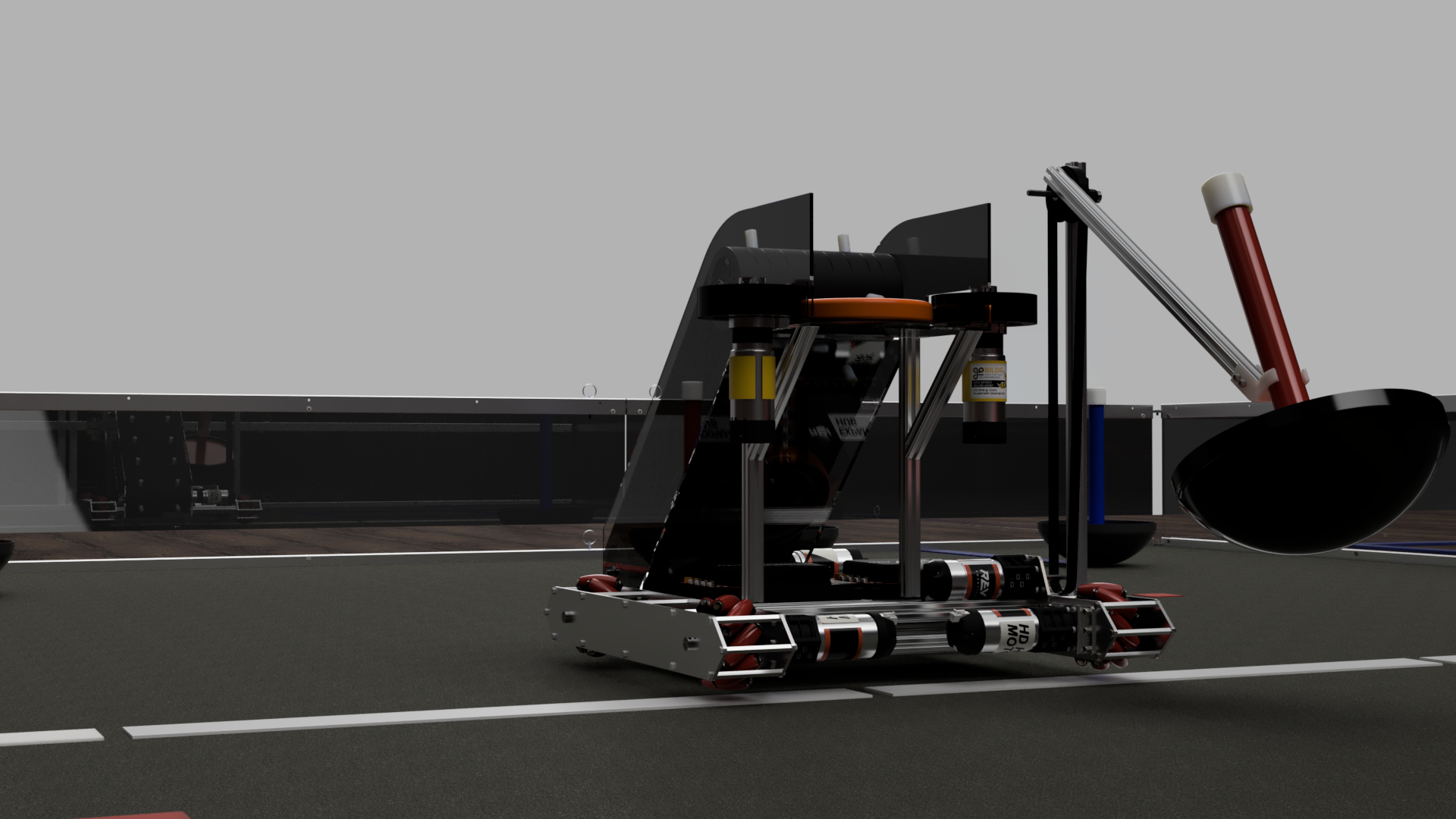
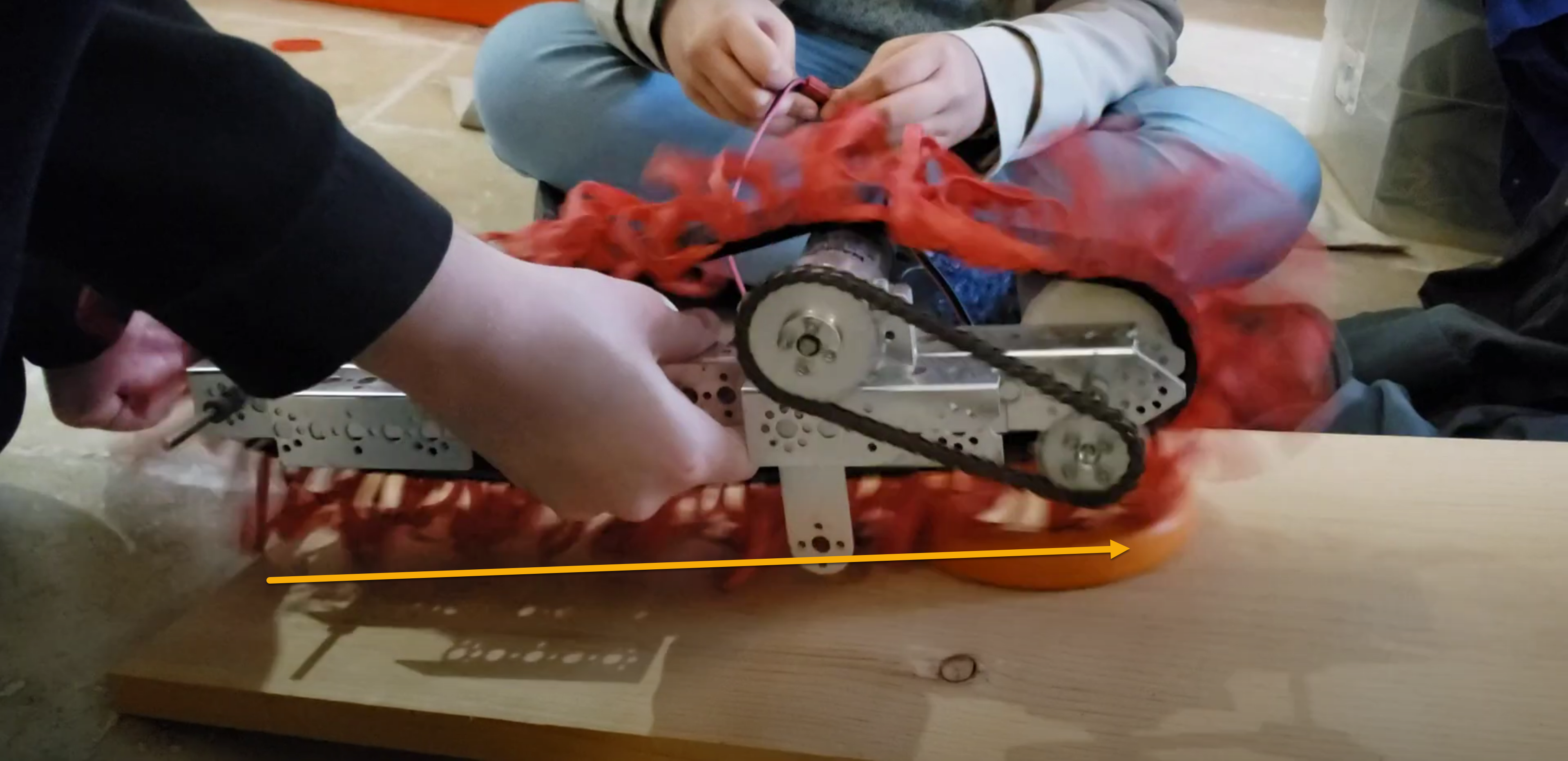
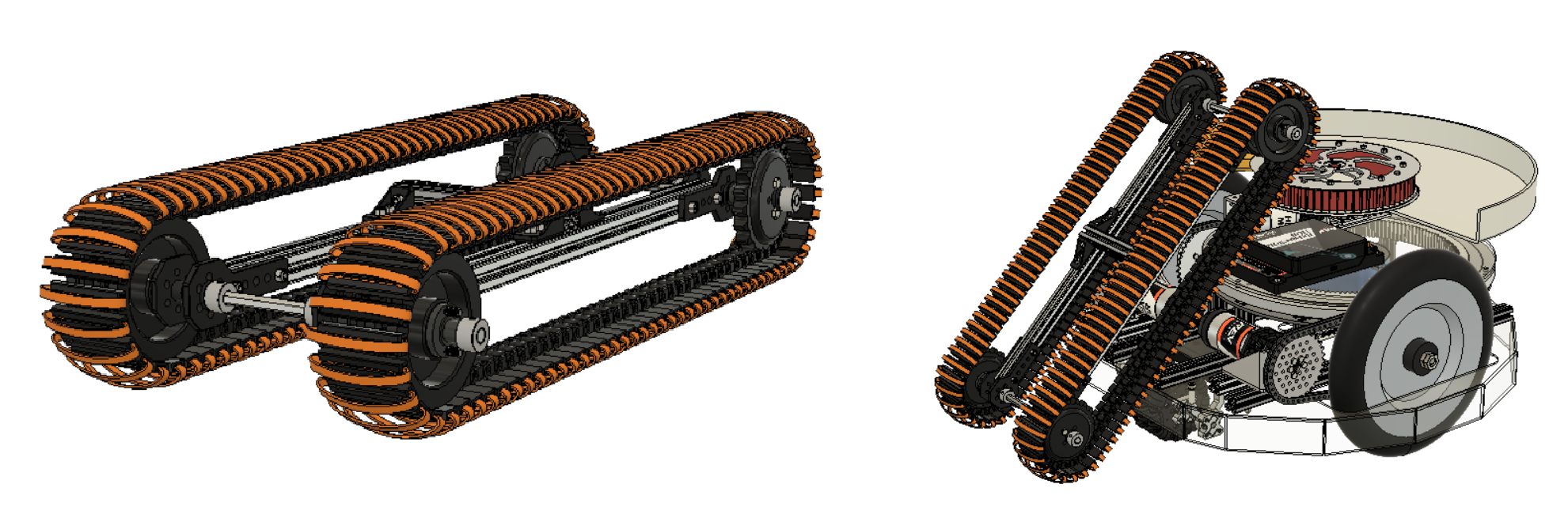
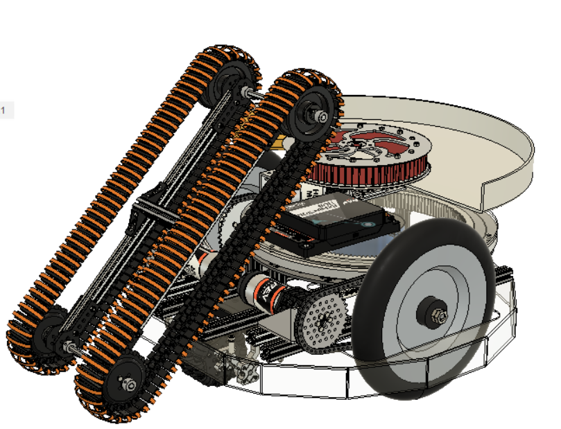
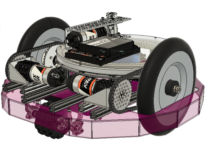
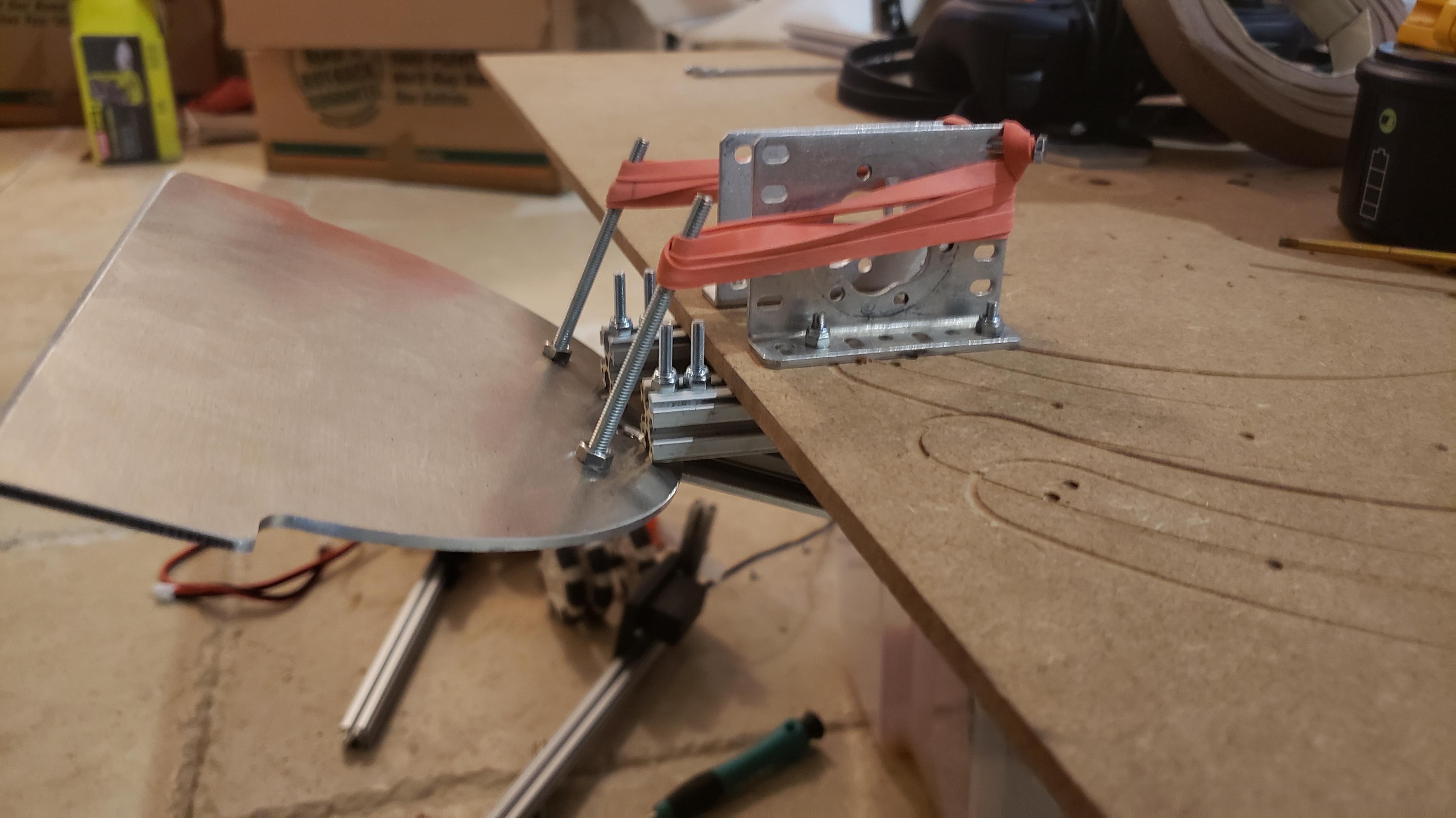
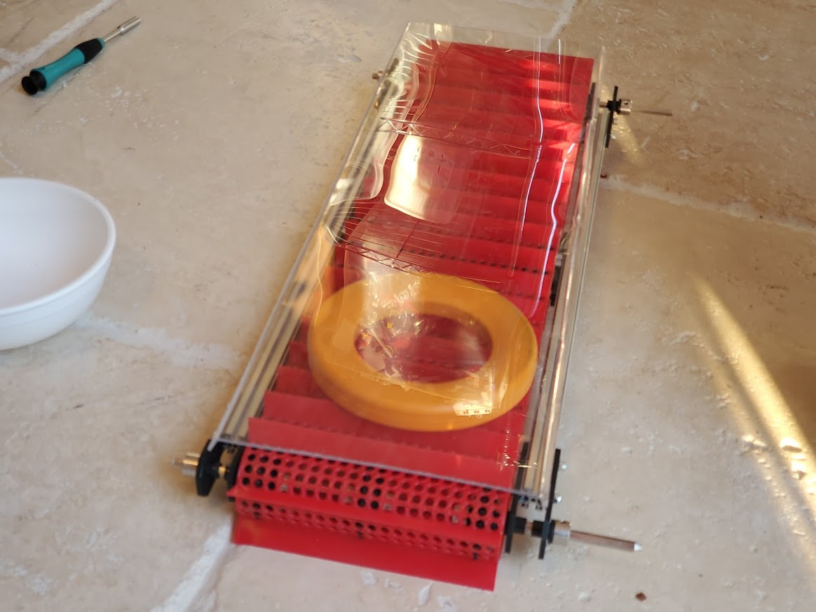
 Since the robot game for this year came out about a week ago, we were thinking about which kind of drive system would work best for the challenge, which mostly involves climbing. Some of the concept we came up with were rocker bogies, rubber-banded tires and a tank drive with treads. Since we already had the preliminary design started for a tank drive, I started modeling that.
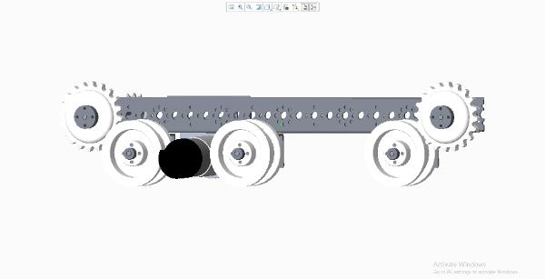
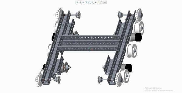
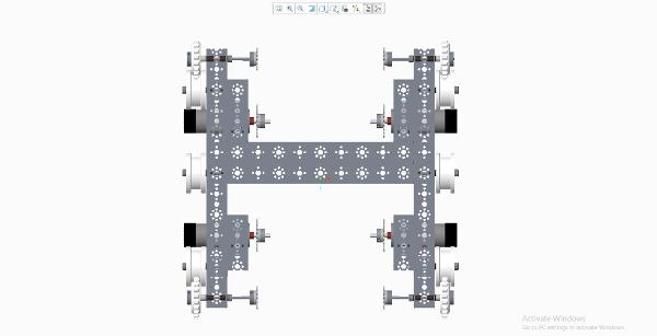
 I also came up with a way to connect both halves of the robot for when we build the left side of our tank drive, and modelled what that would look like when complete.
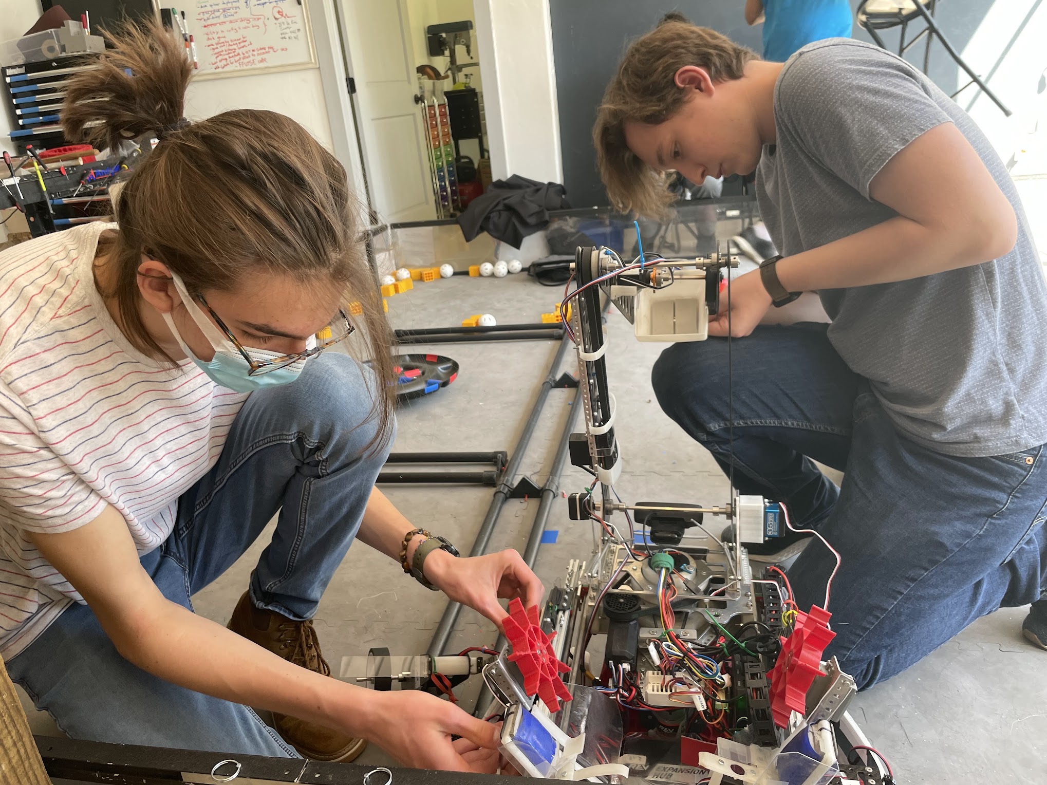
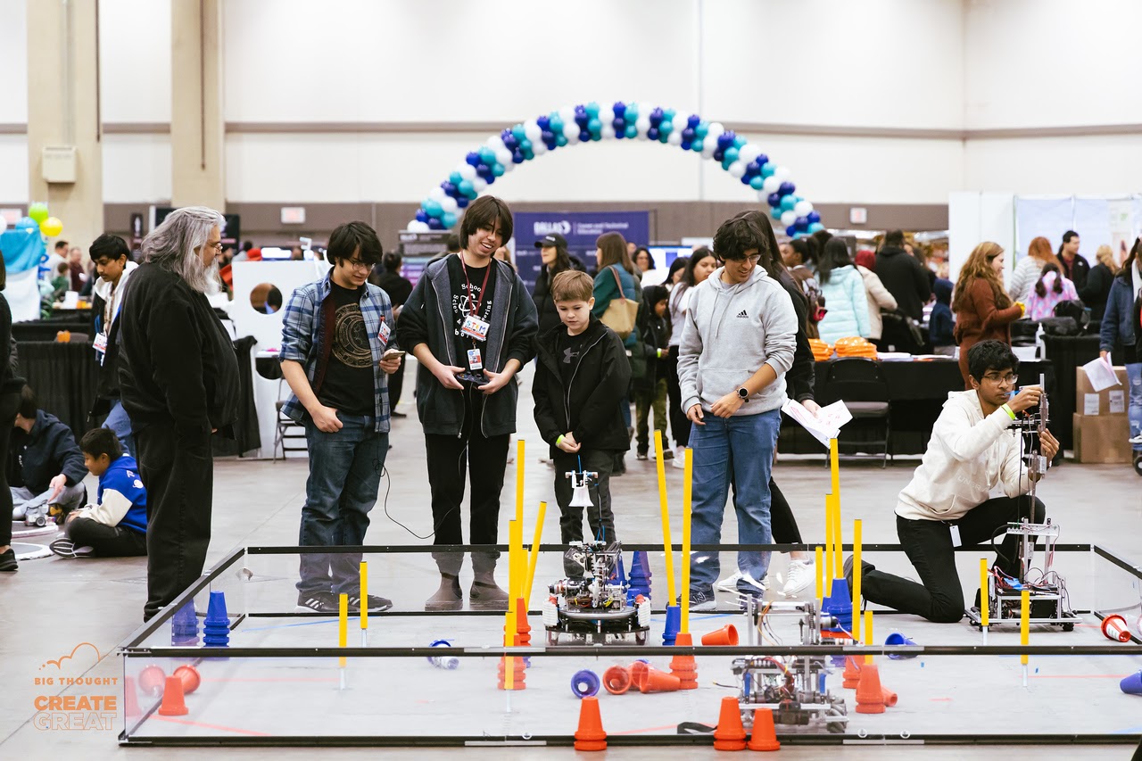
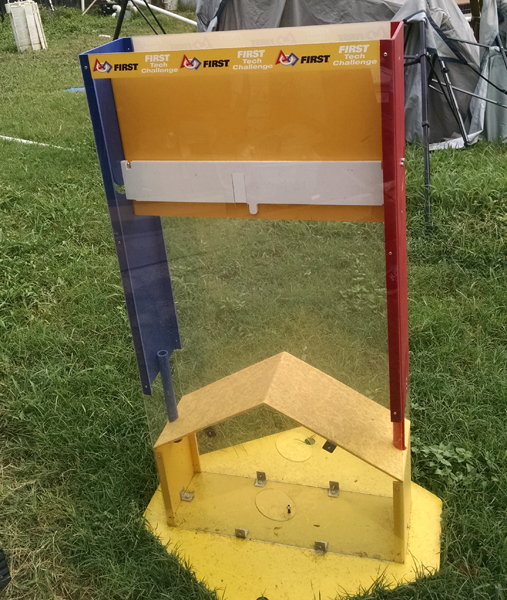
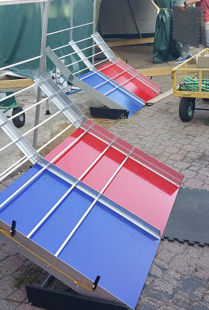
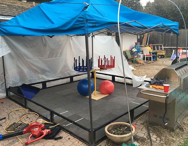
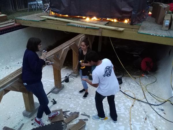
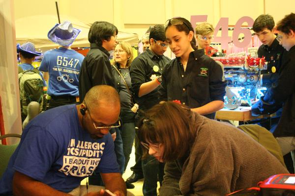
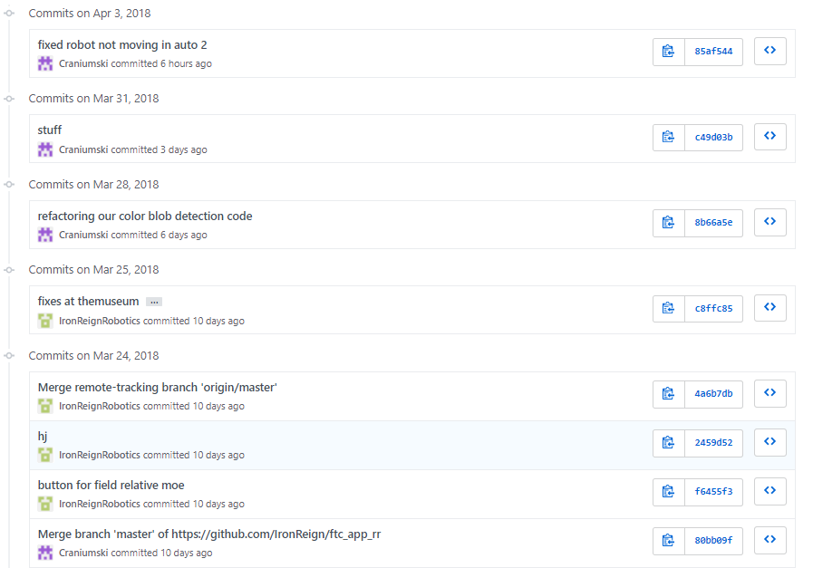
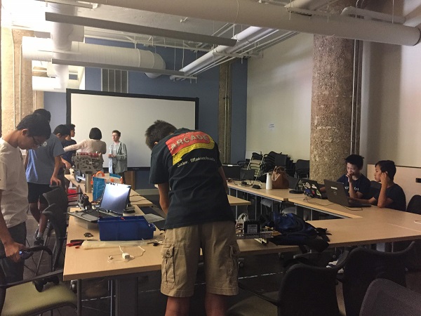
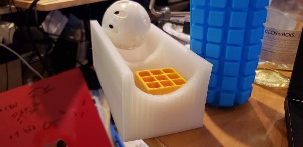
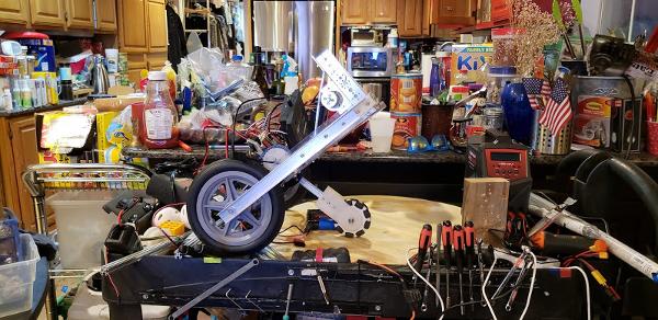
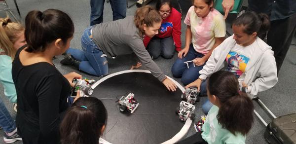
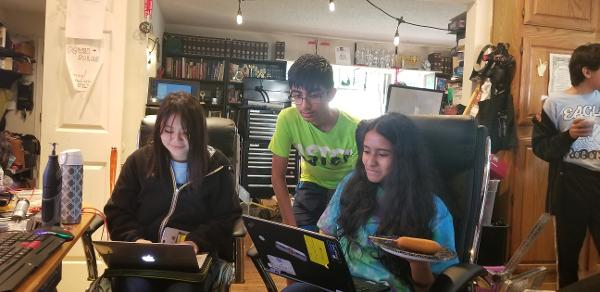
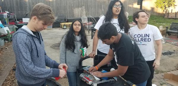
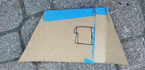
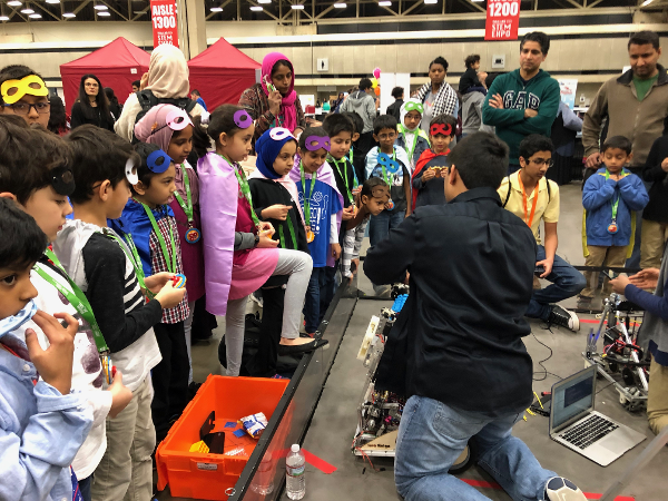
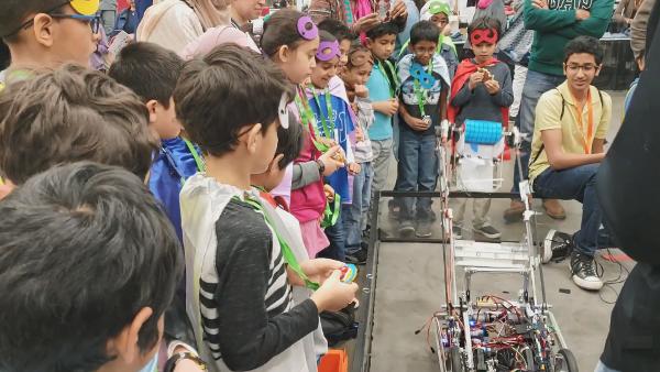
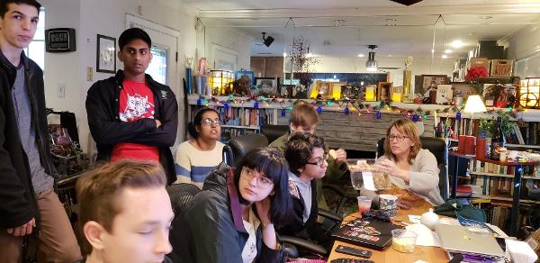
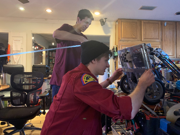
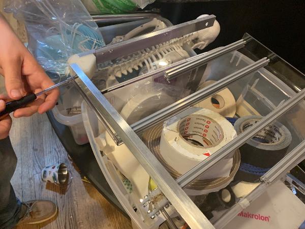
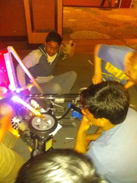
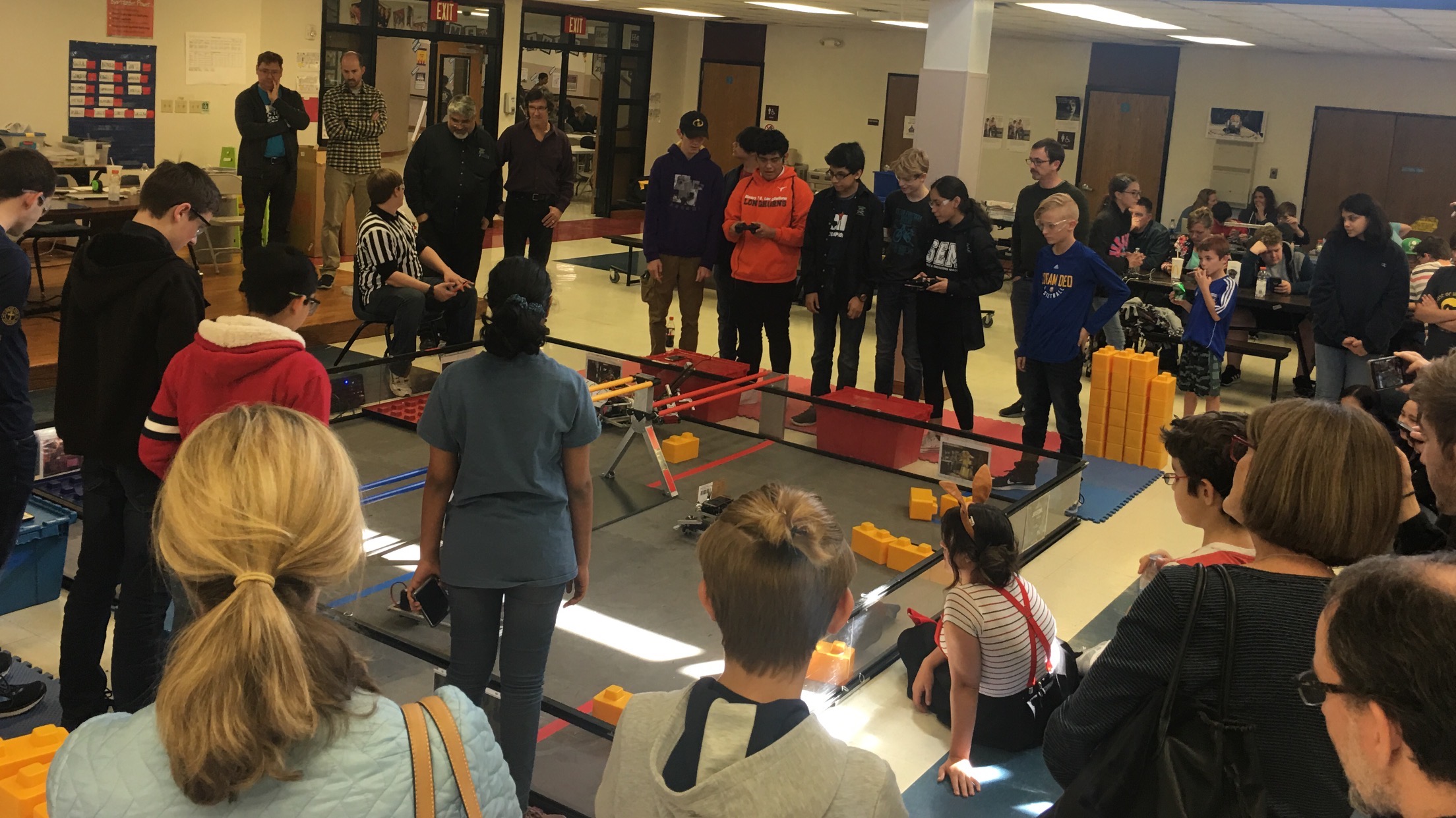
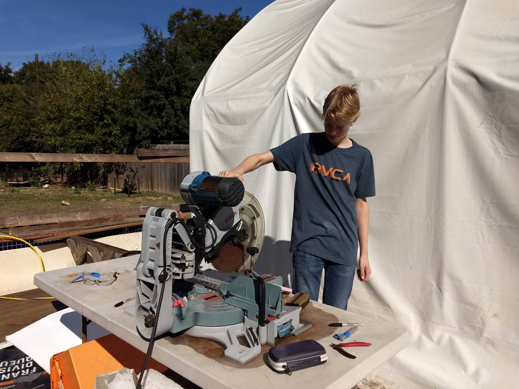
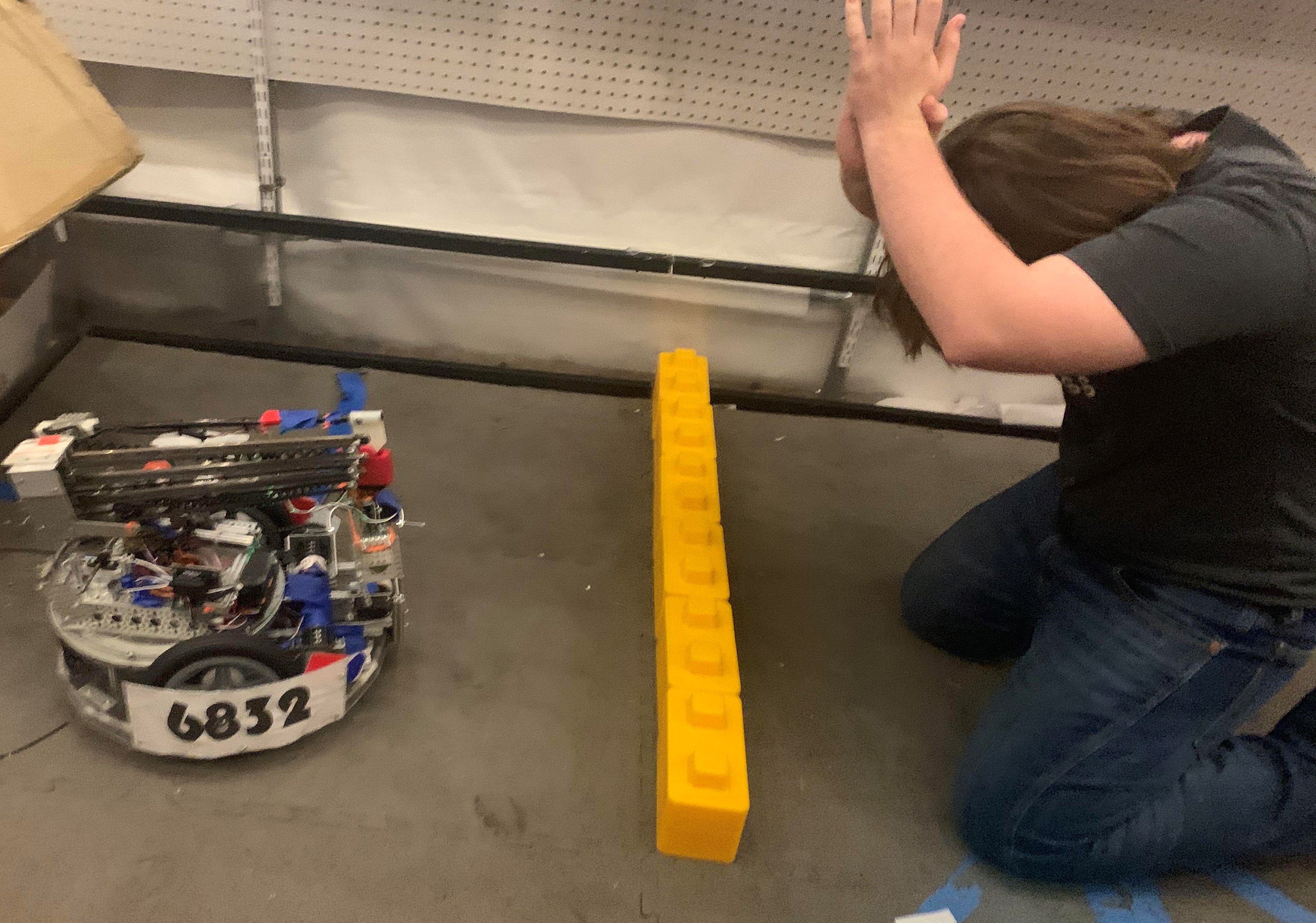
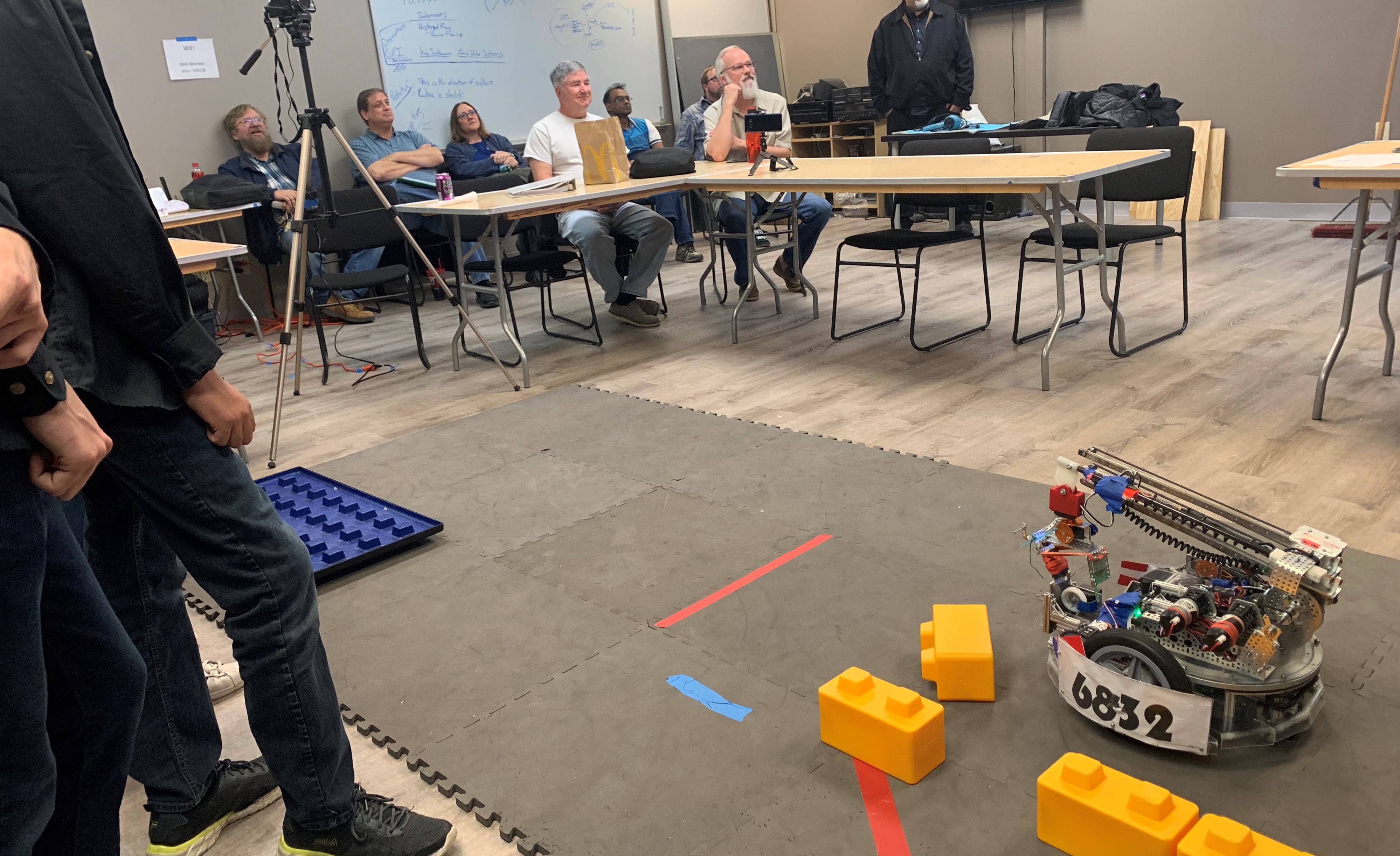
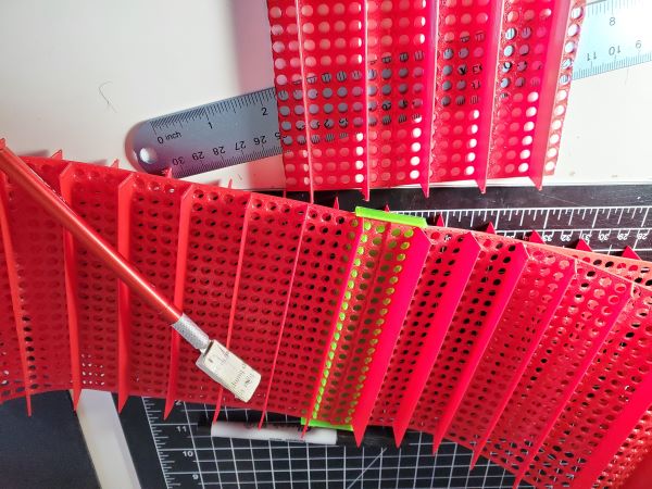
 Today we were charged with the task of building the FTC field. There was one problem. The tent we were setting it up in was in a state of decay. We cleaned out the area to make space while others put together the field. It was changed comletely from when it started. When cleaning we discovered many cool things like cassettes and floppy disks. The mat of the field was a little old but we're going to replace it once we get to the fine tuning of the robot. All in all it was a productice day.

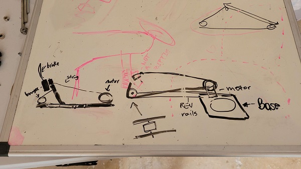
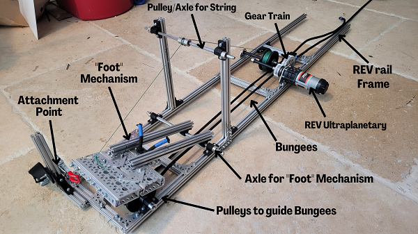
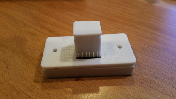
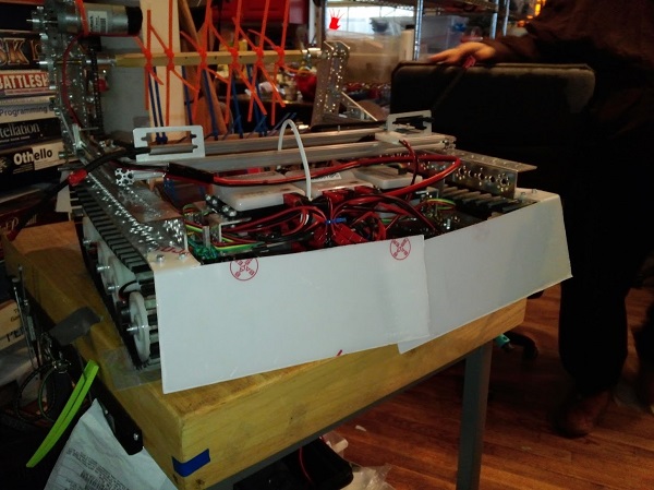
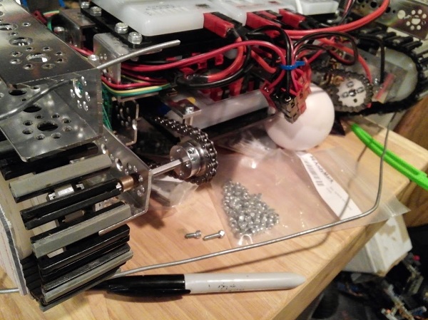
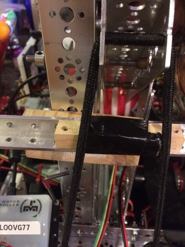
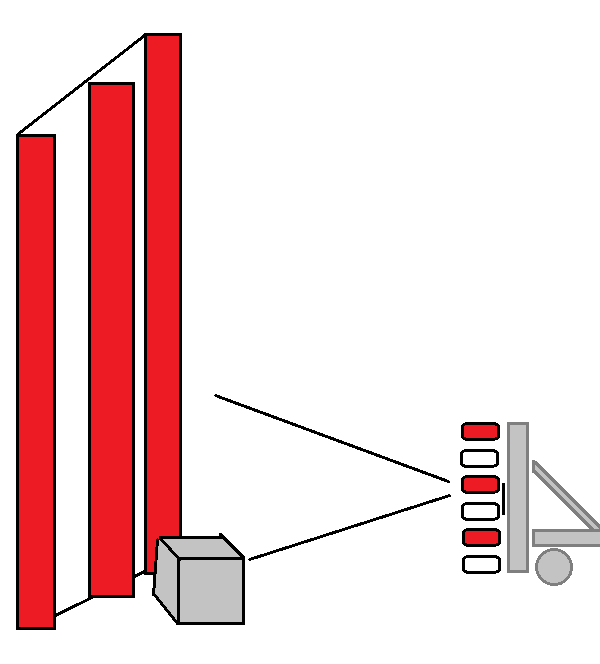
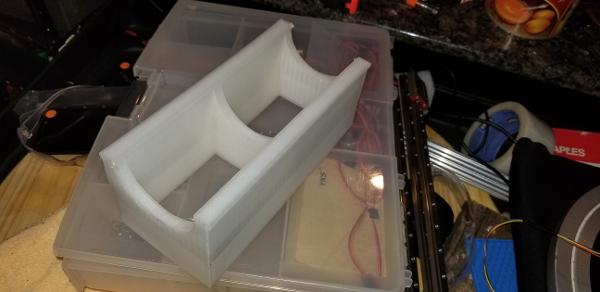
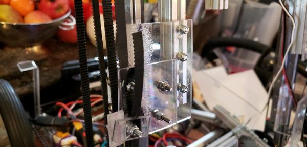
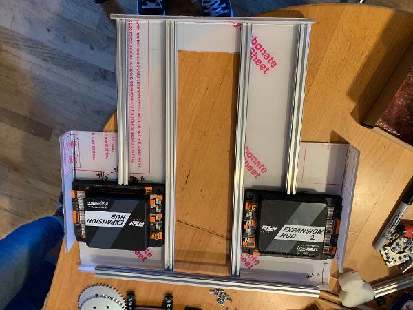
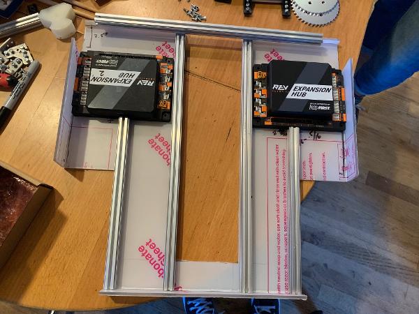
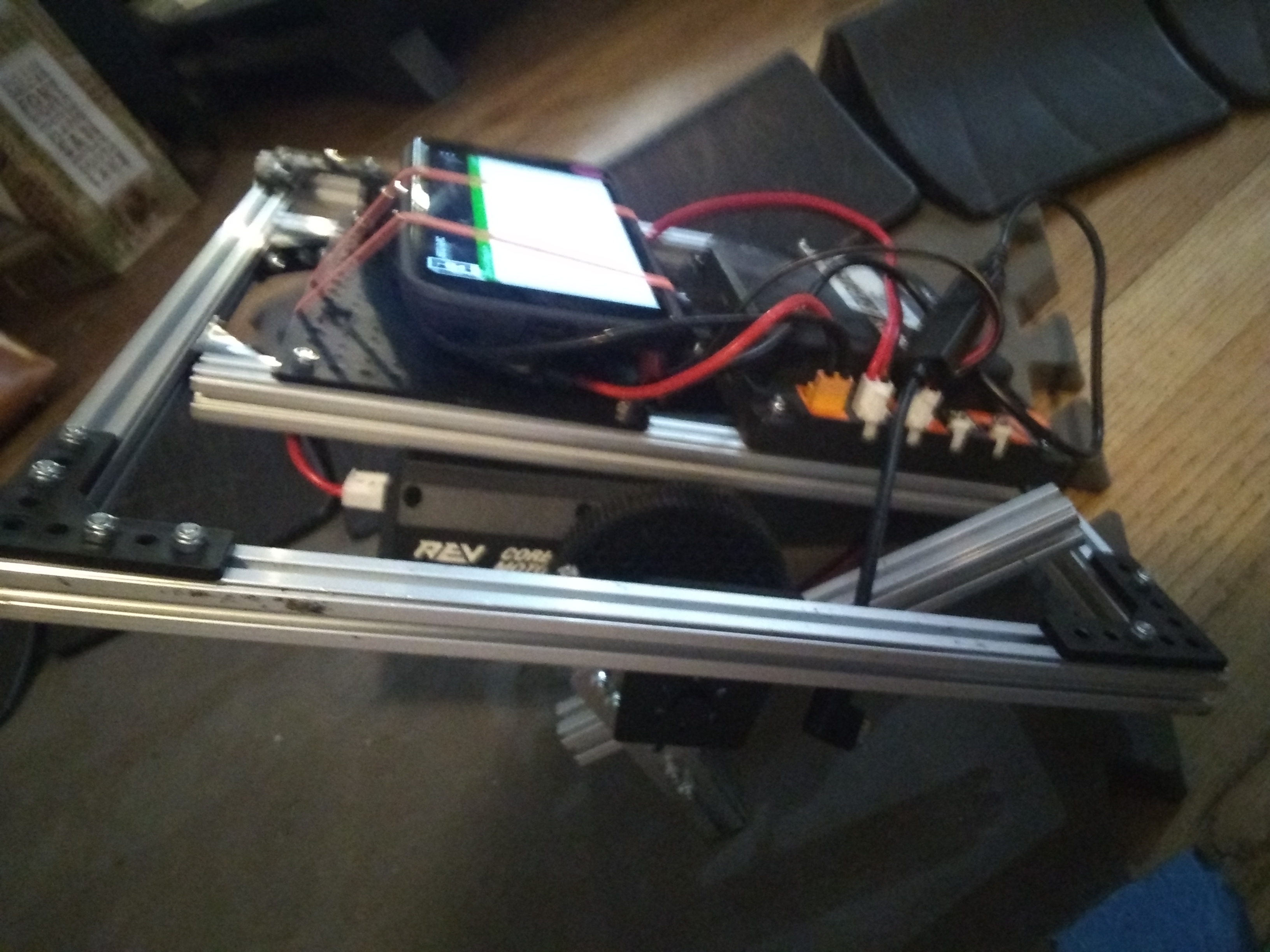
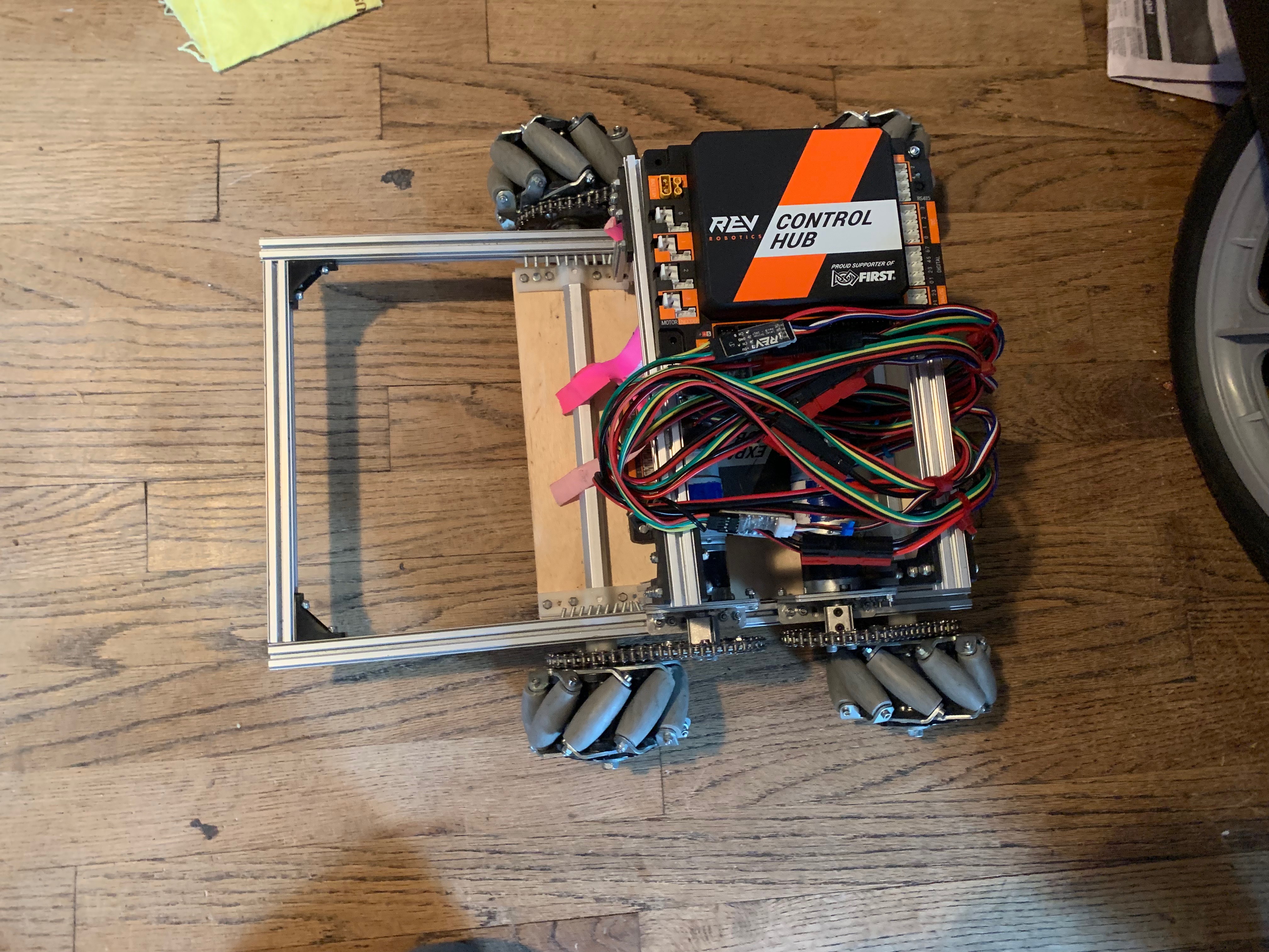
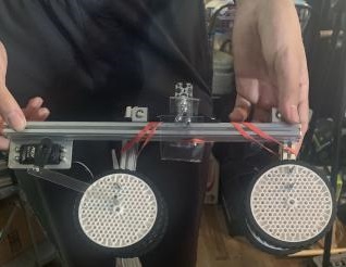
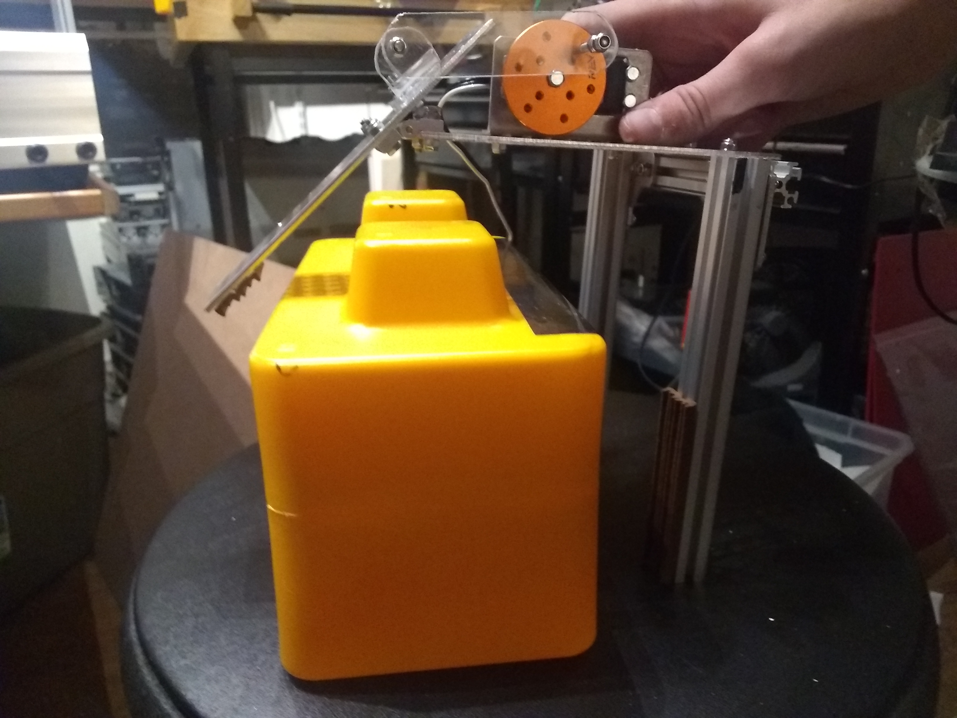
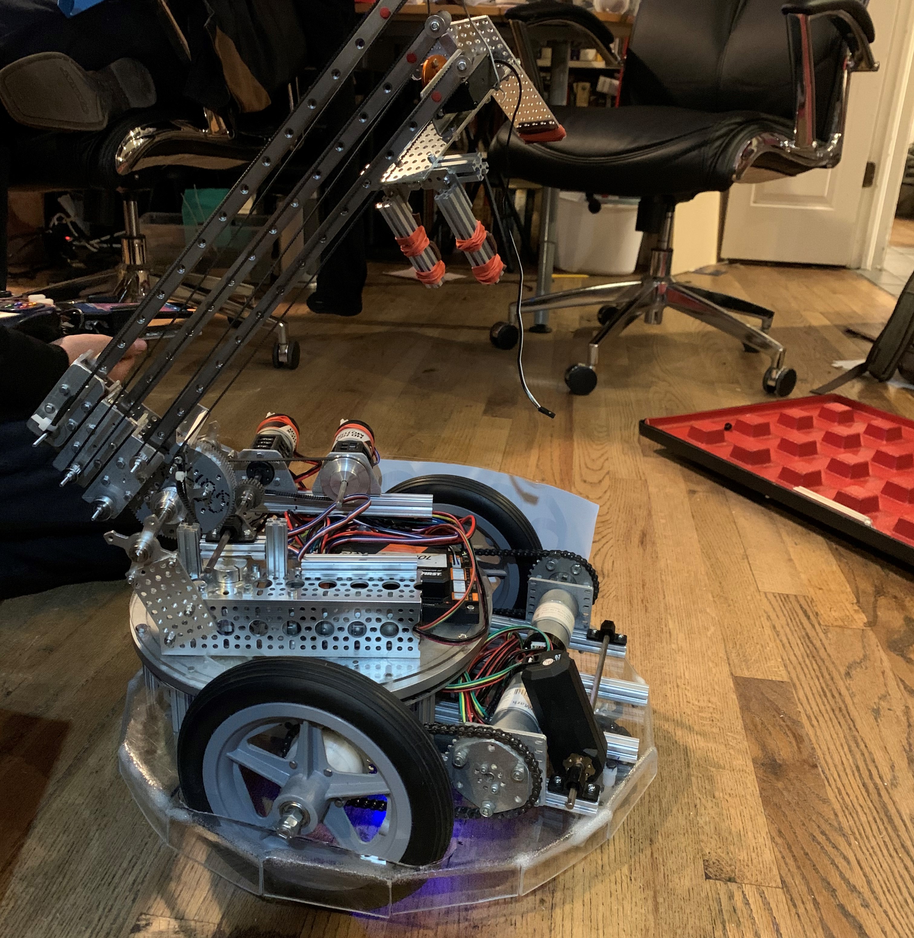
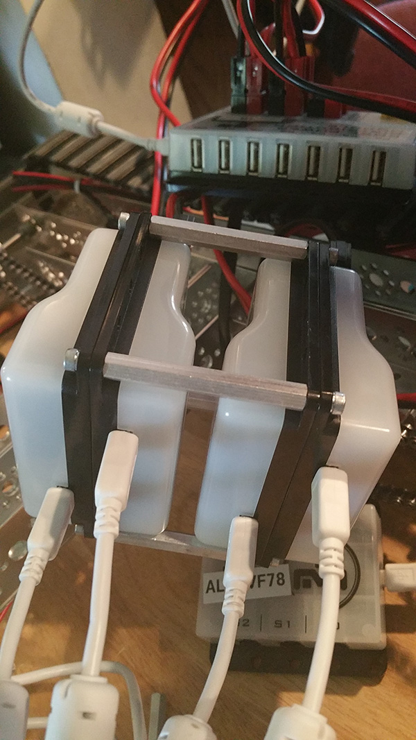 When placed on the robot, this arrangement fit well and did not take up that much vertical space. However, the wires connecting everything were
packed up inside and were ungainly, so we took it apart and started over. The next arrangement we came up with was this: (INSERT PICTURE HERE LATER)
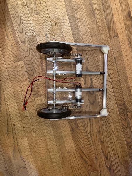
This one takes very little vertical space, but no longer fits inside the robot and is quite long.
When placed on the robot, this arrangement fit well and did not take up that much vertical space. However, the wires connecting everything were
packed up inside and were ungainly, so we took it apart and started over. The next arrangement we came up with was this: (INSERT PICTURE HERE LATER)
This one takes very little vertical space, but no longer fits inside the robot and is quite long.
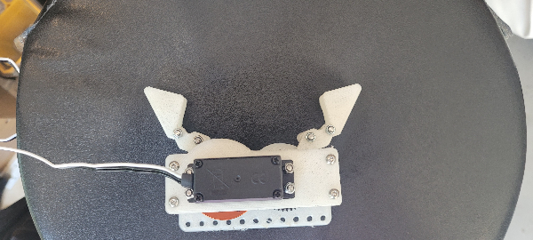
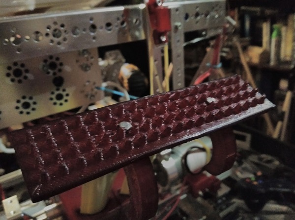
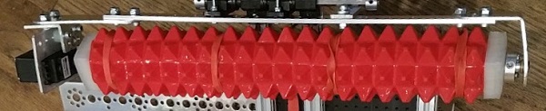
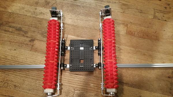
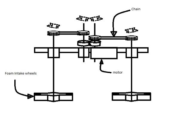
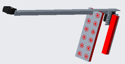
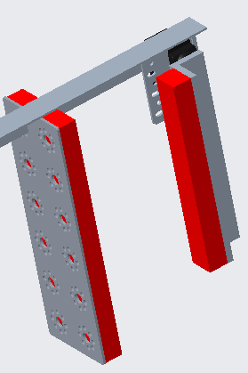
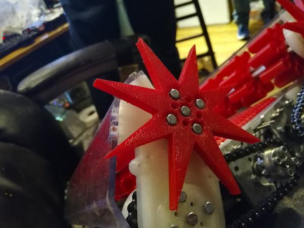
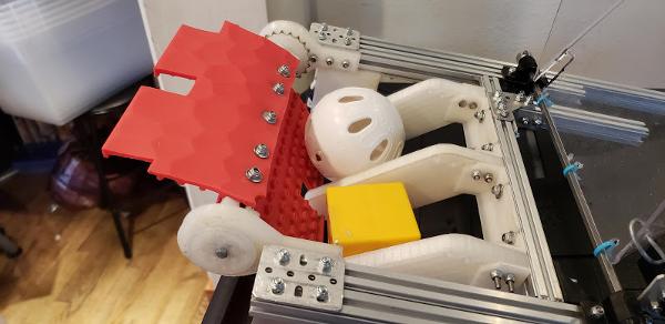
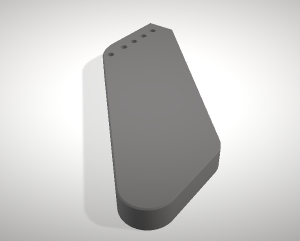
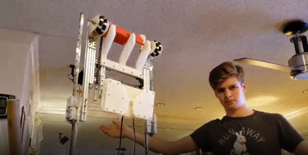
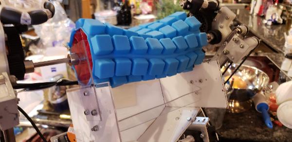
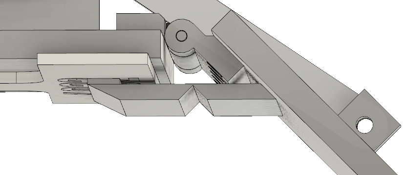
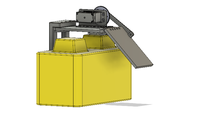
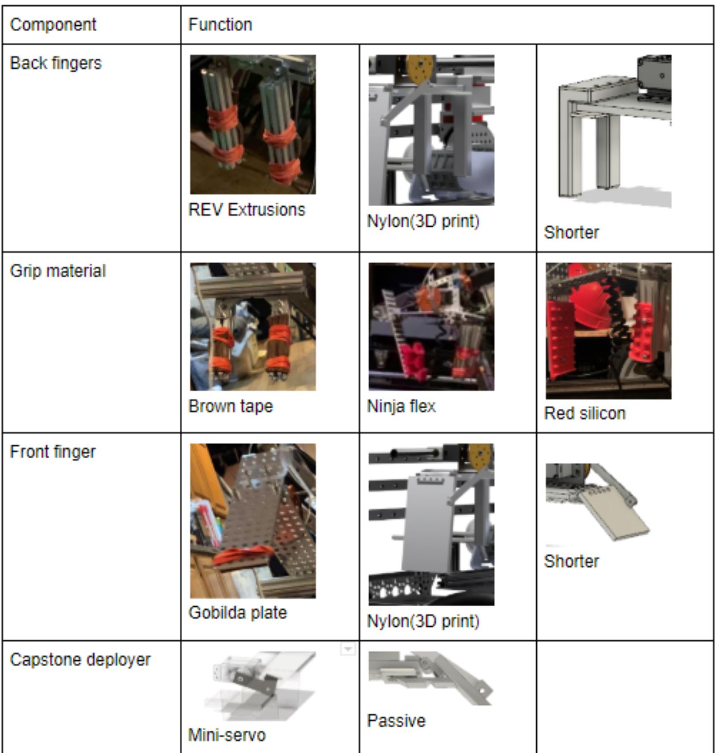
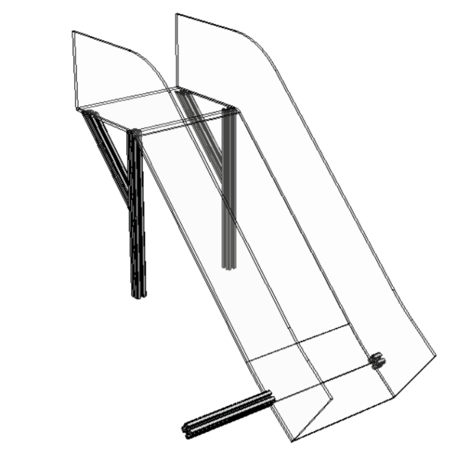
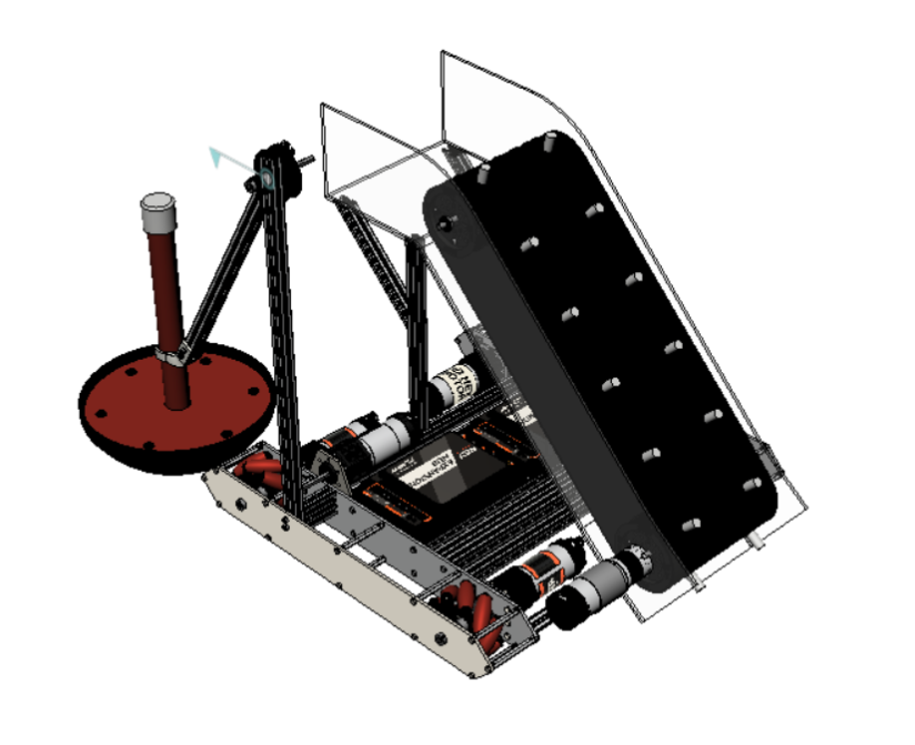
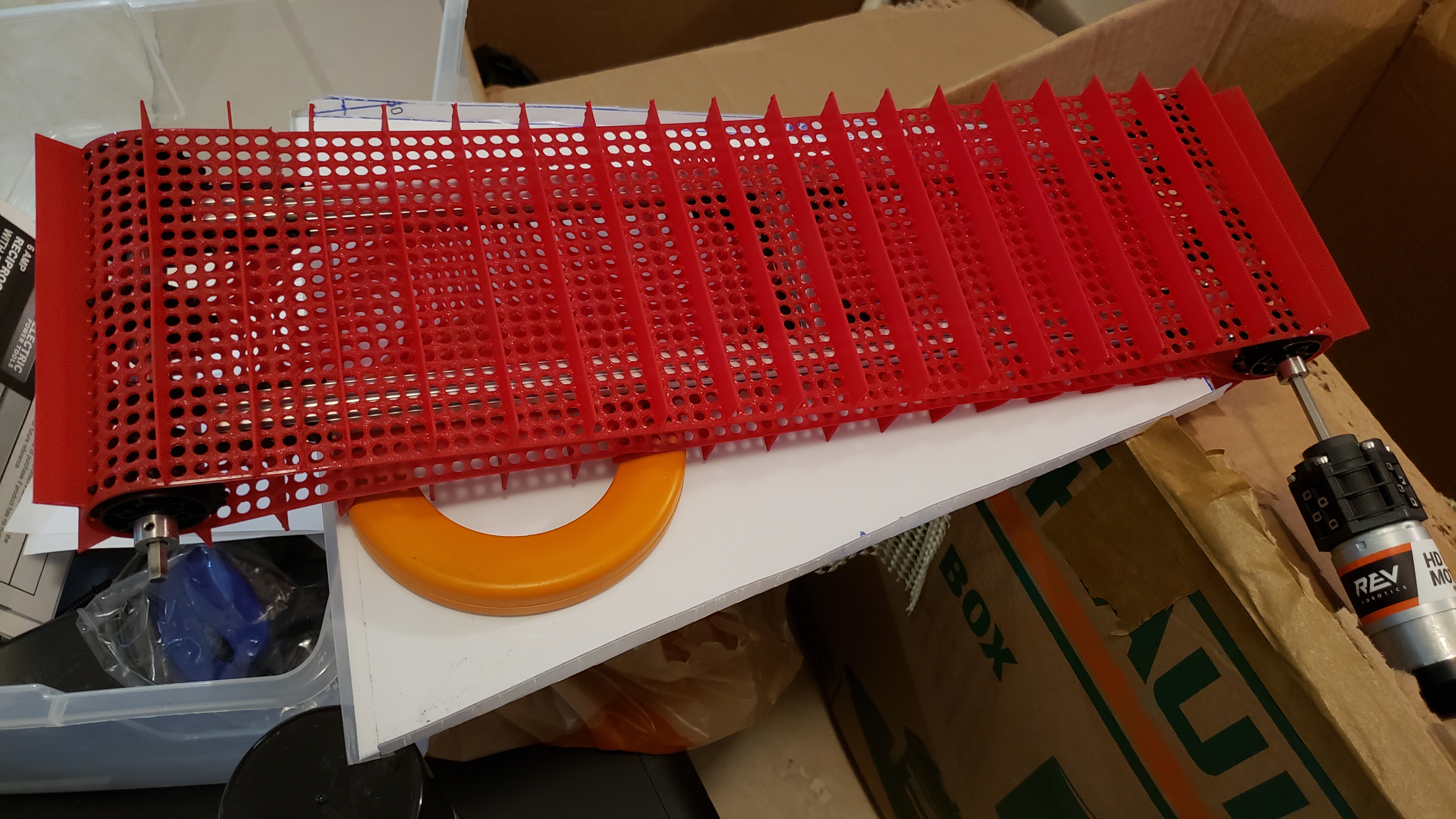
 The small plates on the front of each of the sides are meant to guide the beater bar's sliding off the robot when being deployed.


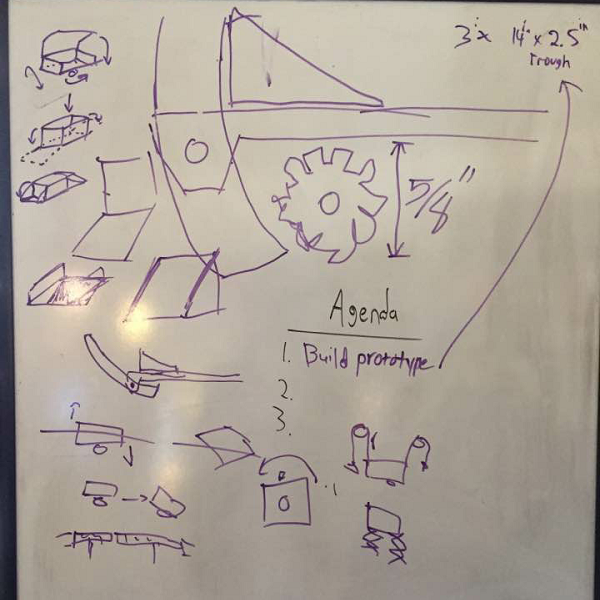
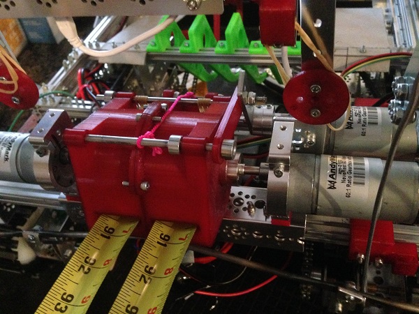
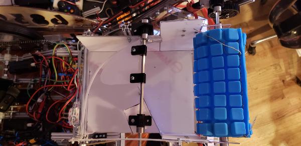
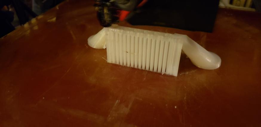
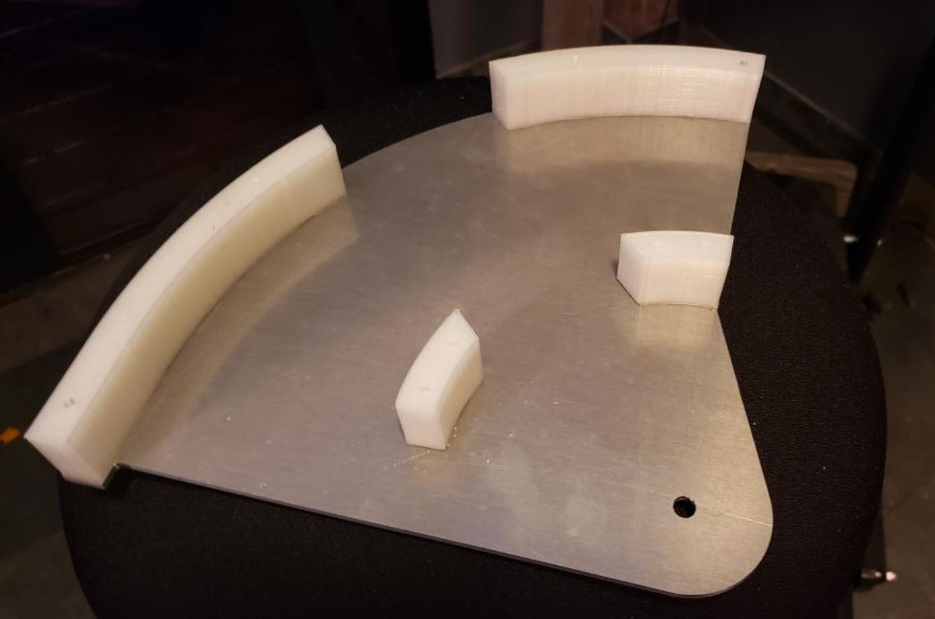
 We also 3D-printed and installed a couple of things (Max-designed): first, small guides that the arms can move through so that they push forward and pull back the way we want them to; and second, longer pieces that hold the beater bar back while it's waiting to be released.
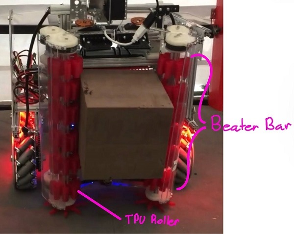
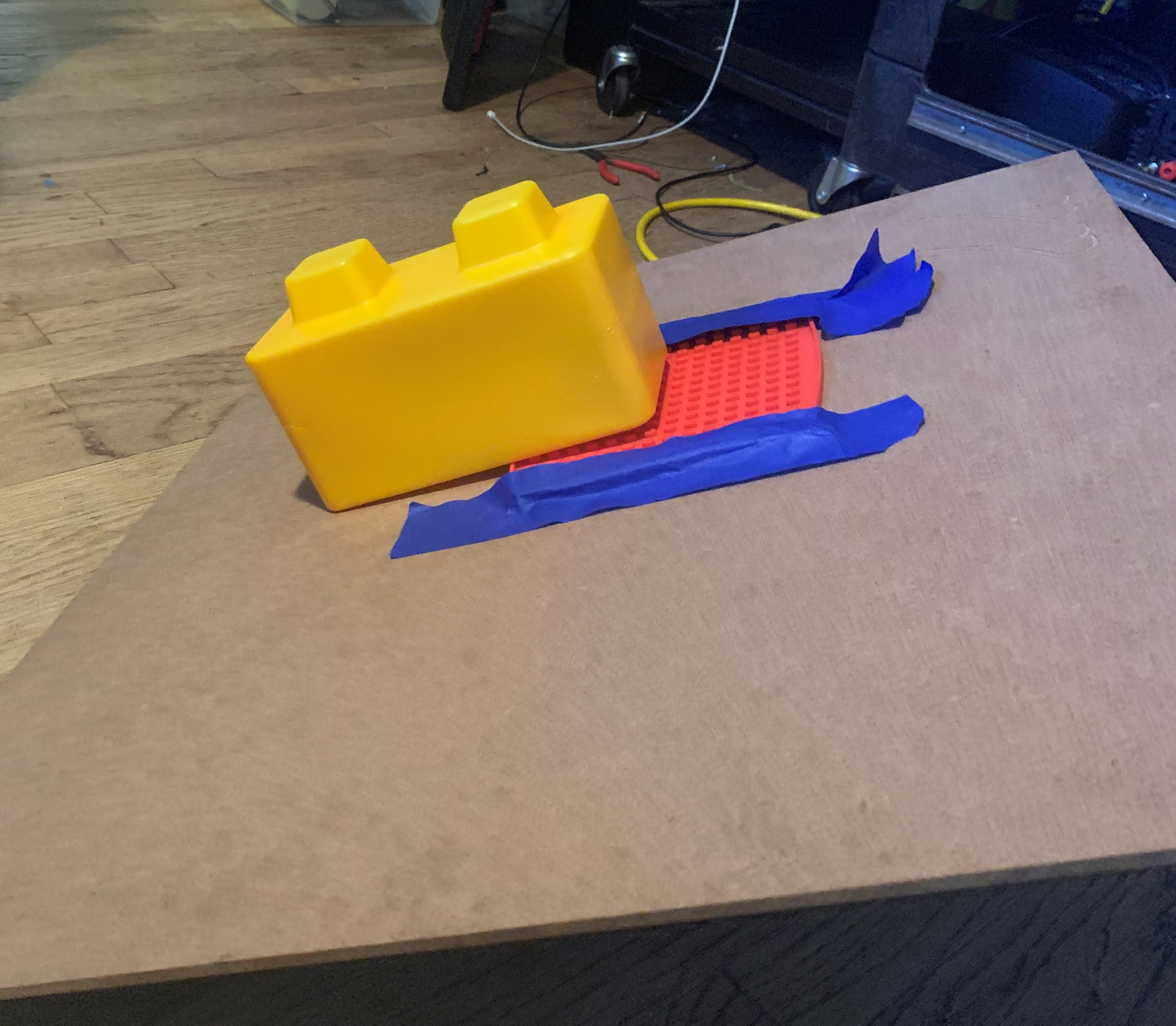
 As a small quality-of-life improvement, we have added a couple of pieces of cardboard to the sides of the beater bar today to block game elements from getting stuck in the empty spaces that are there.
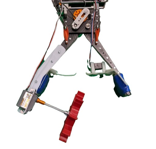
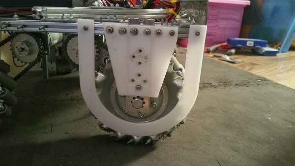
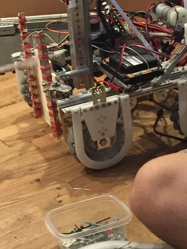
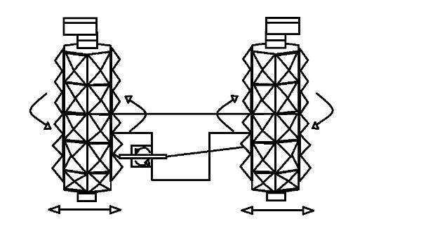
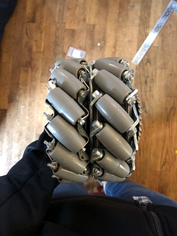
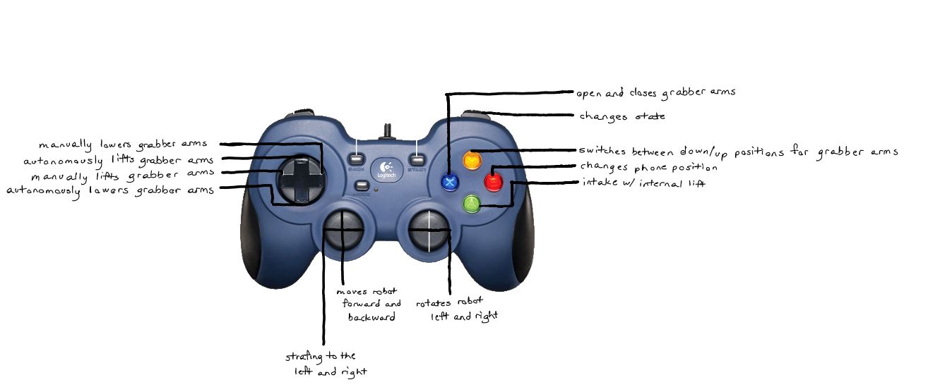
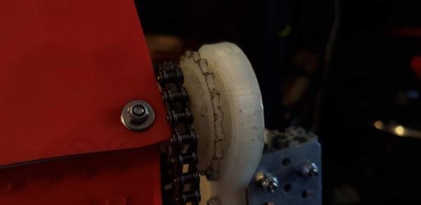
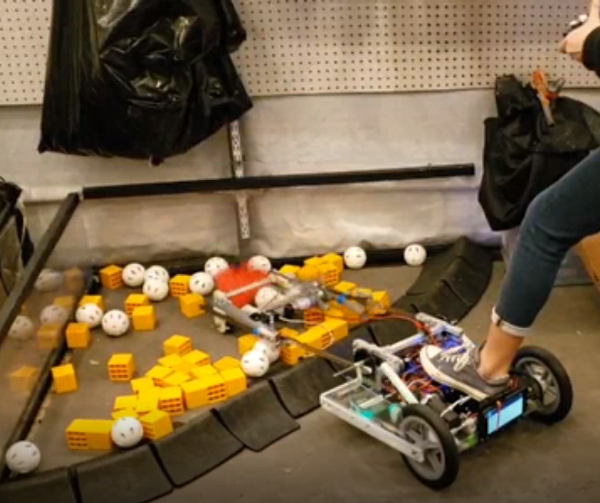
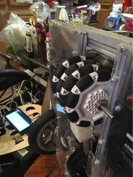
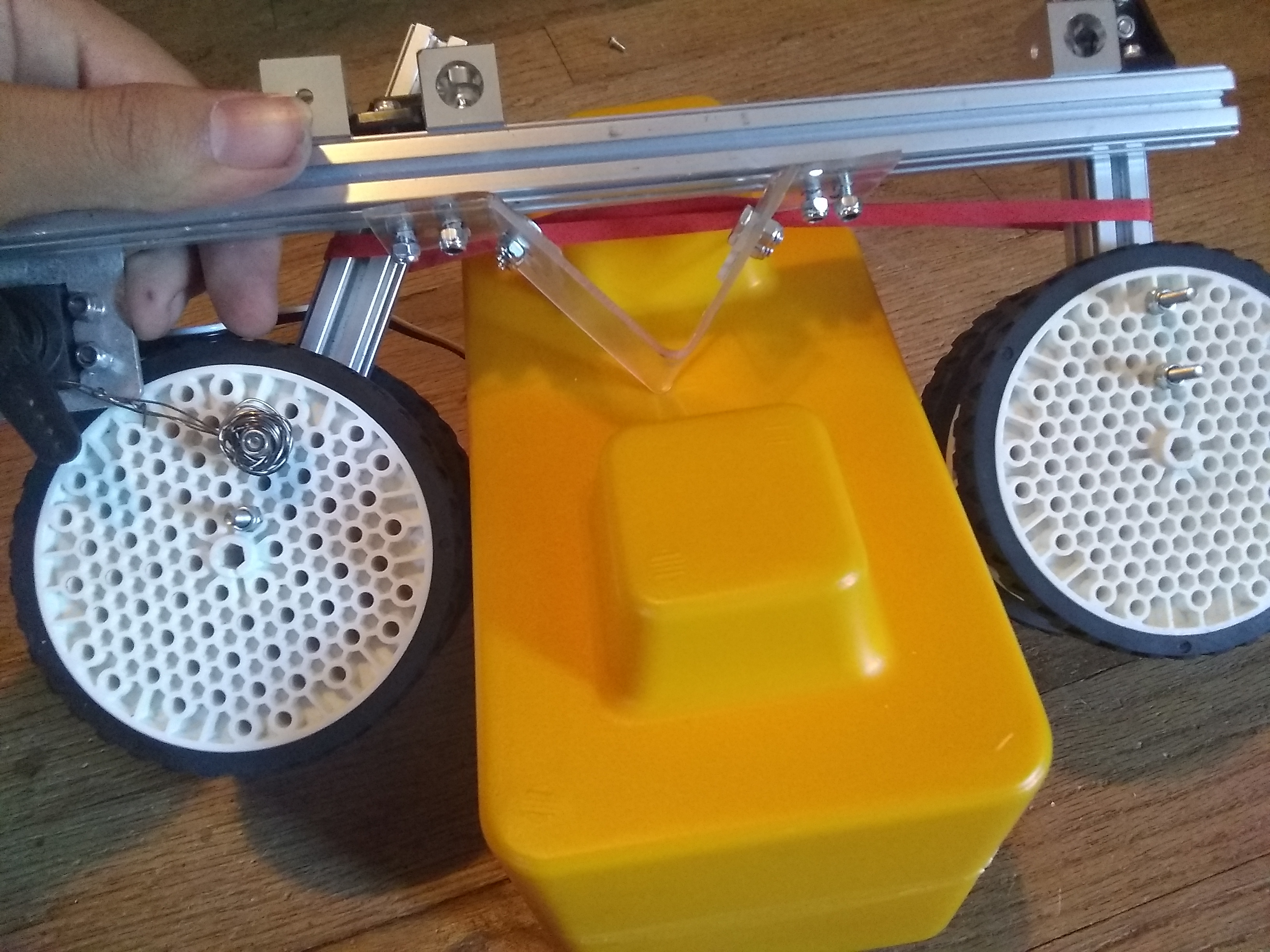
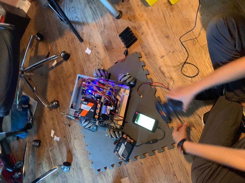
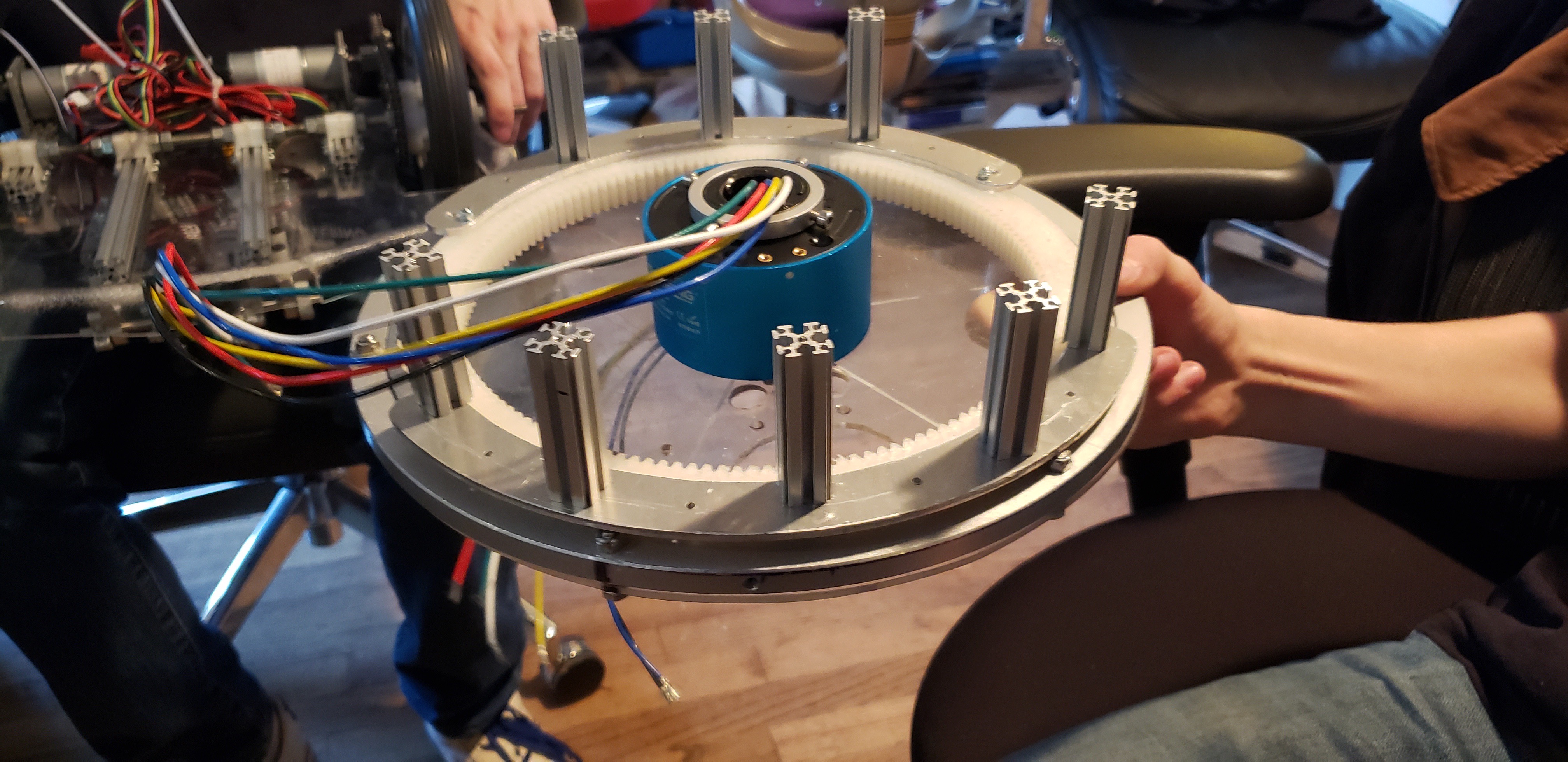
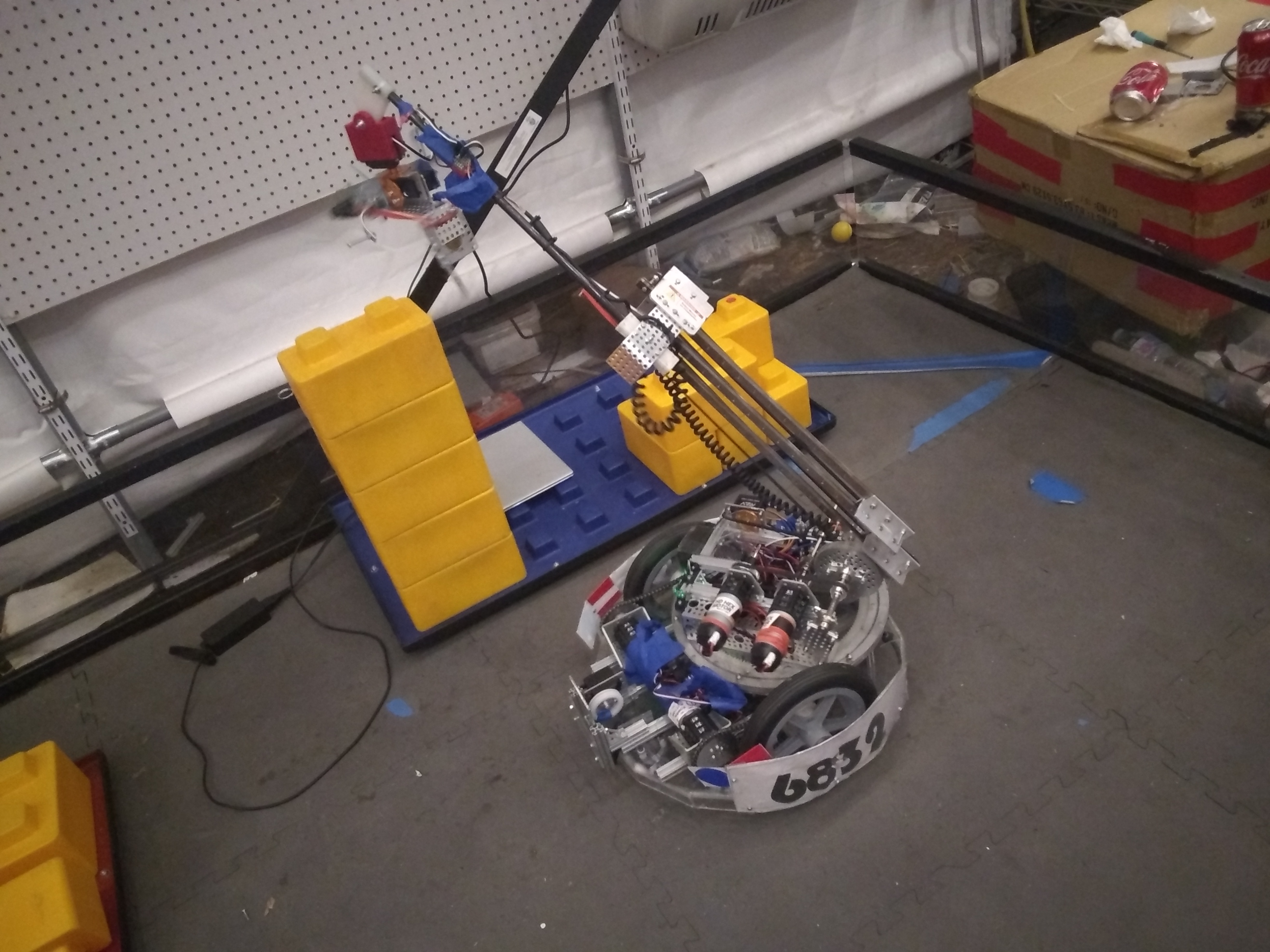
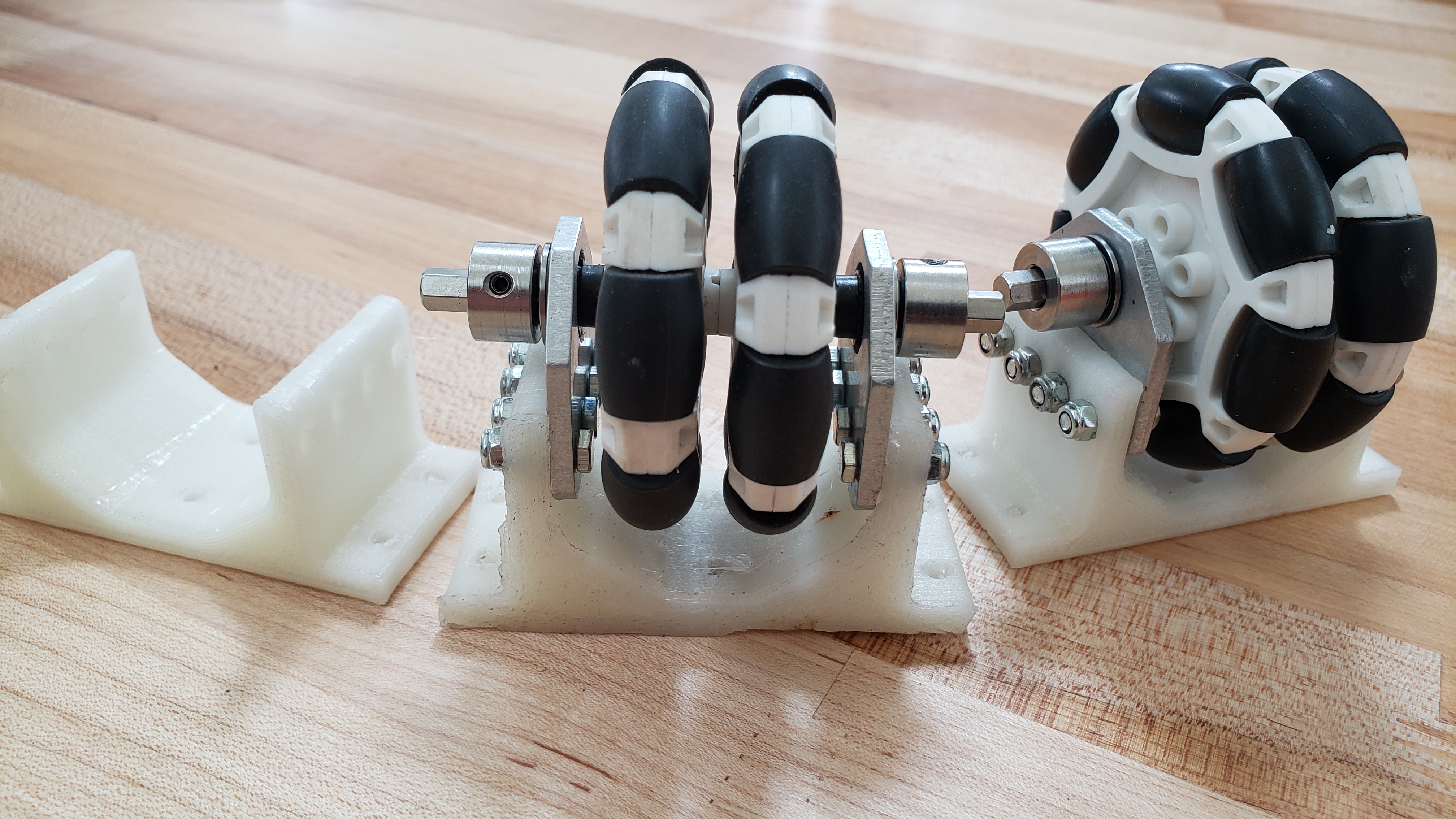
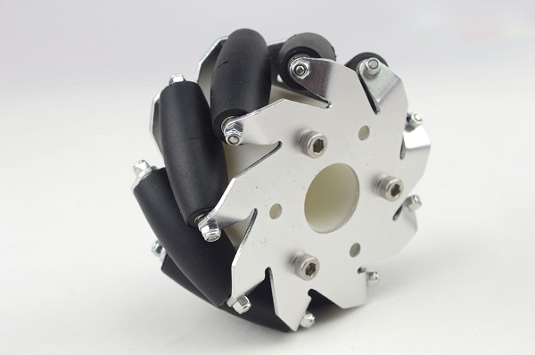 The cool thing about these wheels is that they enable you to strafe side to side, instead of turning. However, they do require different coding than our normal wheels.
 This is important, because if these wheels are not pointing in the proper direction, then the rollers will begin to fight against each other, causing strange driving patterns that aren't very useful. We learned this the hard way, because when reconstructing the wheel mounts, the positions of two wheels on robot were flipped, causing the robot to drive in circles when we tried to drive sideways.
 However, moving side to side is not really intuitive compared to the others. In order to move side to side, the wheels on either side have to move opposite of each other. For example, if I wanted to, from a top-down perspective, drive to the right, the wheels on the left side of the robot would have to drive away from each other, while the wheels on the right side of the robot would have to drive towards each other. The rollers start spinning away from the center and to the right on the left side of the robot, or towards the center and to the right for the right side of the robot. The forwards and backwards components of the wheels and the rollers cancel each other out, and the robot moves to the right.
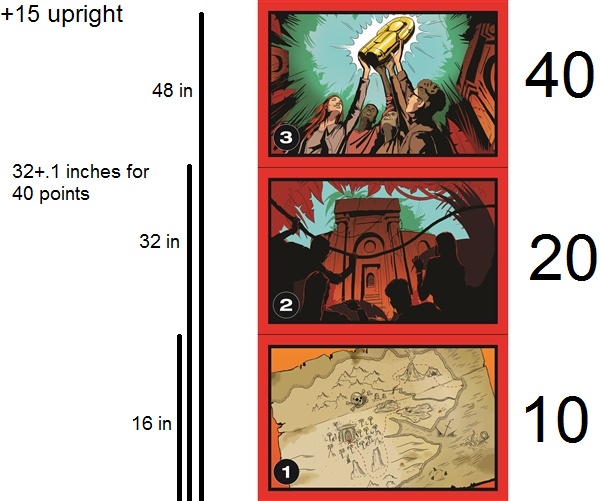
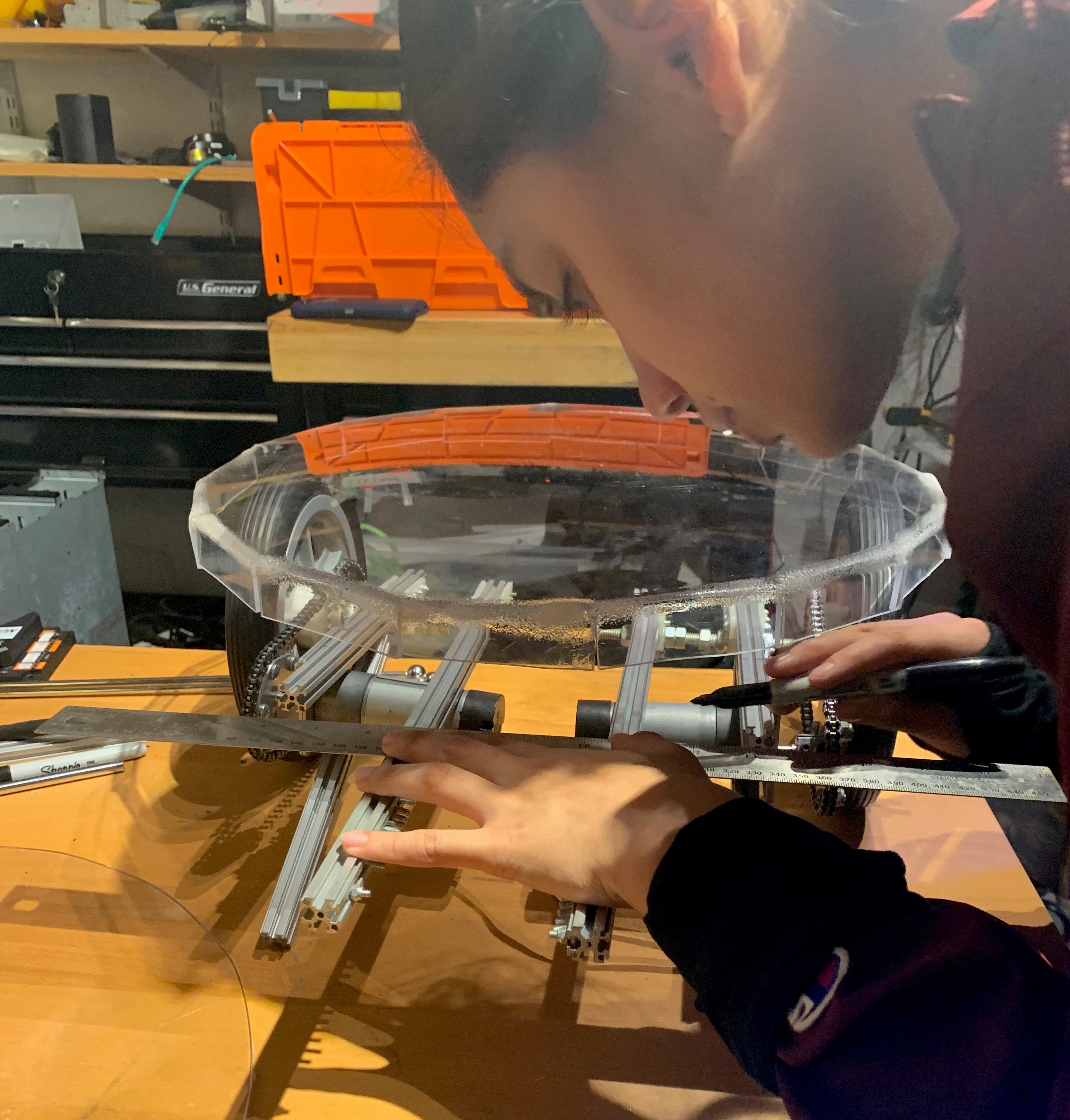
 (herecomedatbowl.jpg)
 (We went with a mix of both)
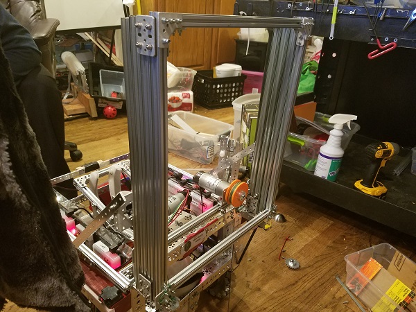
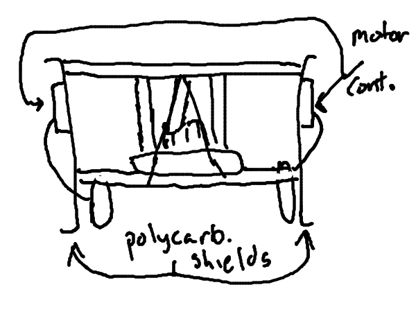
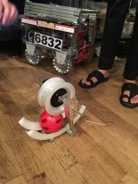
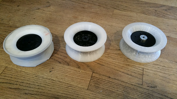

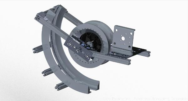
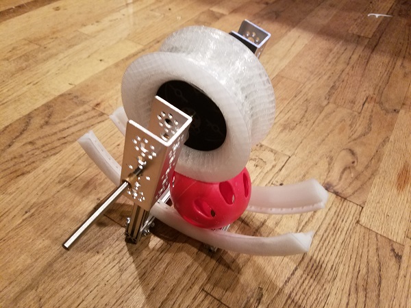
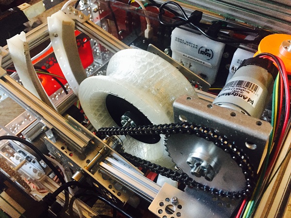

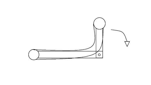
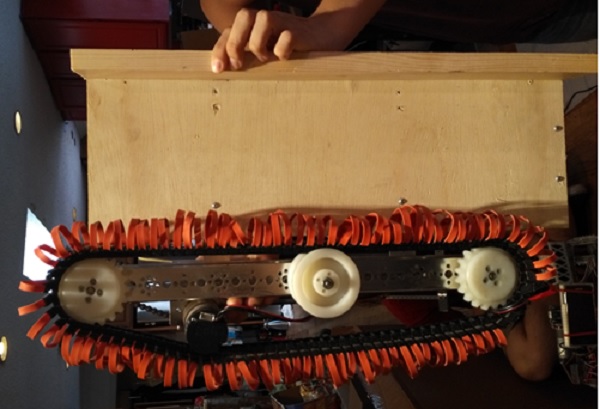

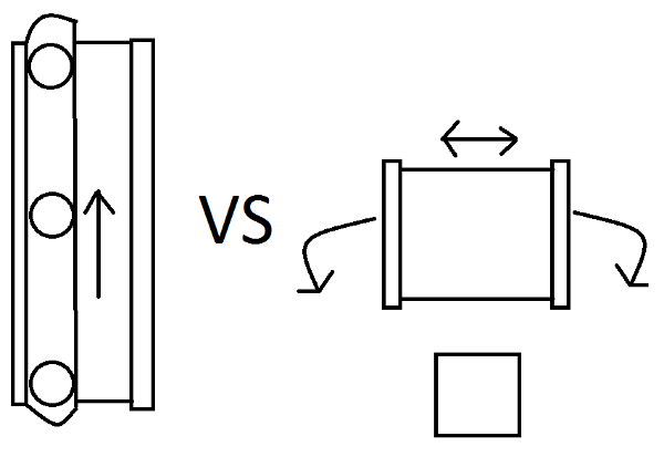
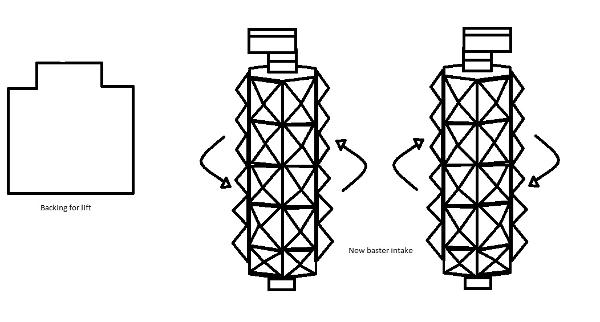
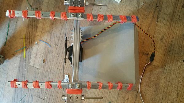
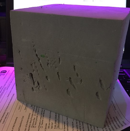
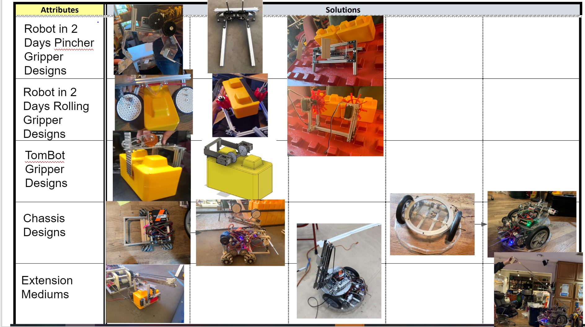
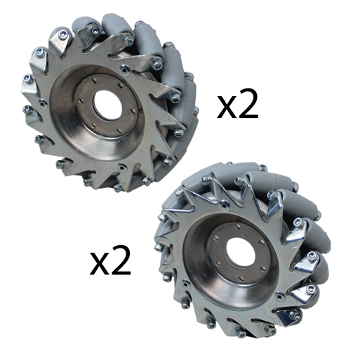 Fig 2
Fig 2
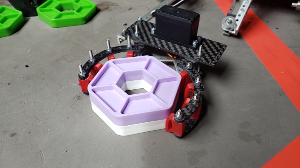
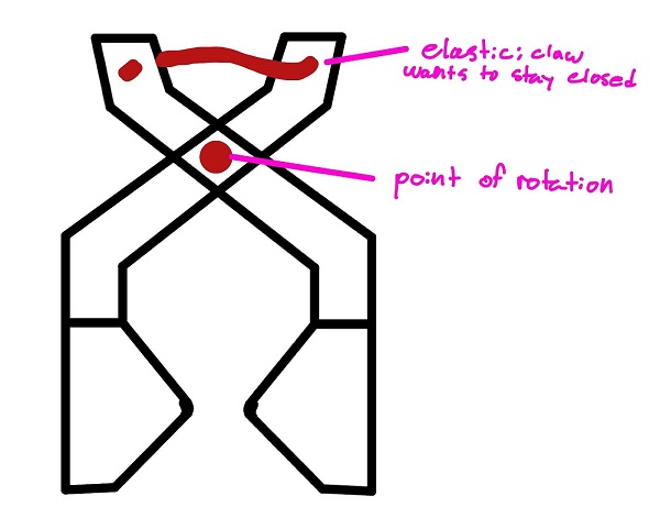
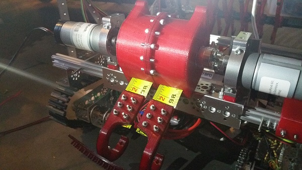
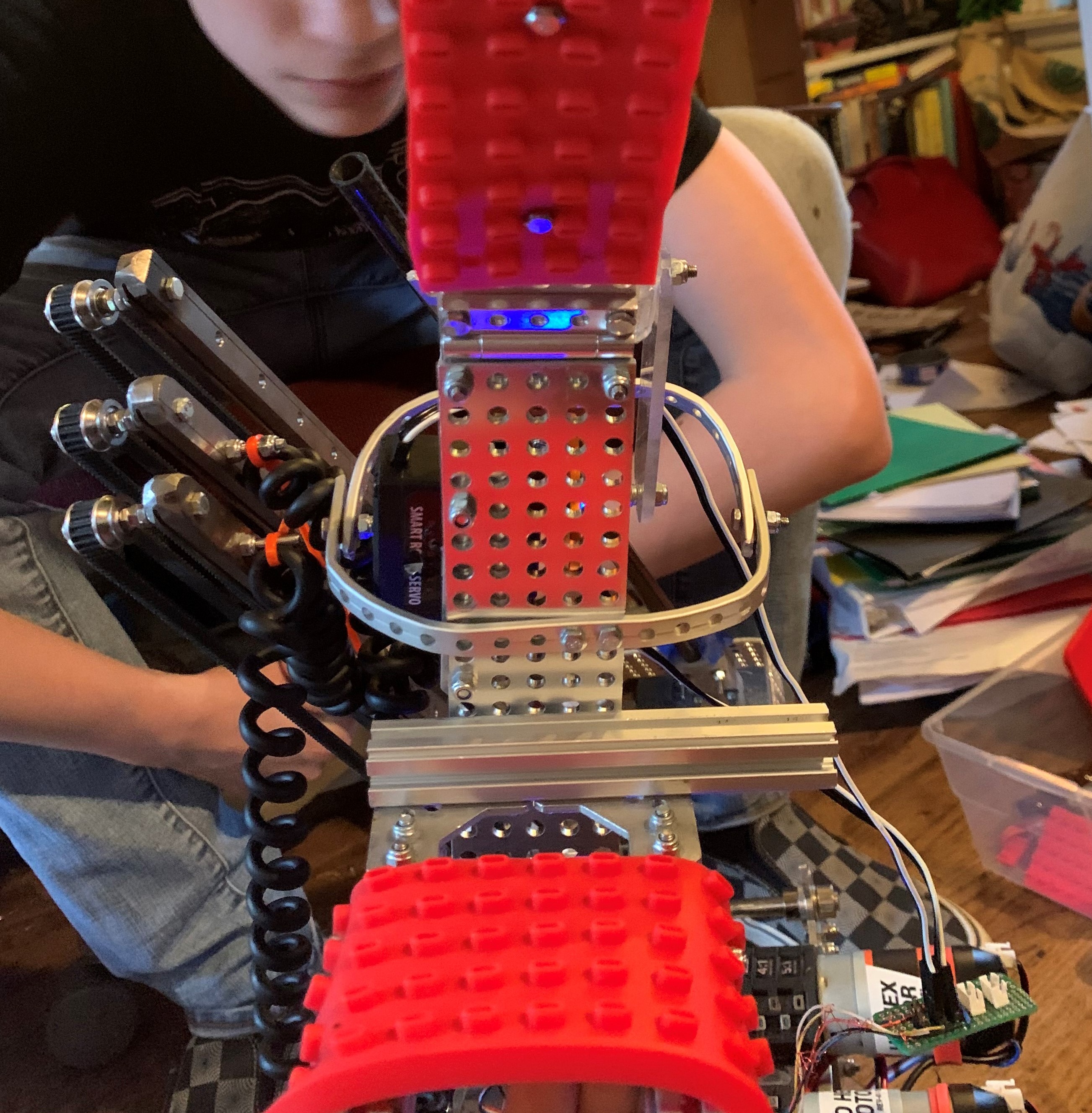
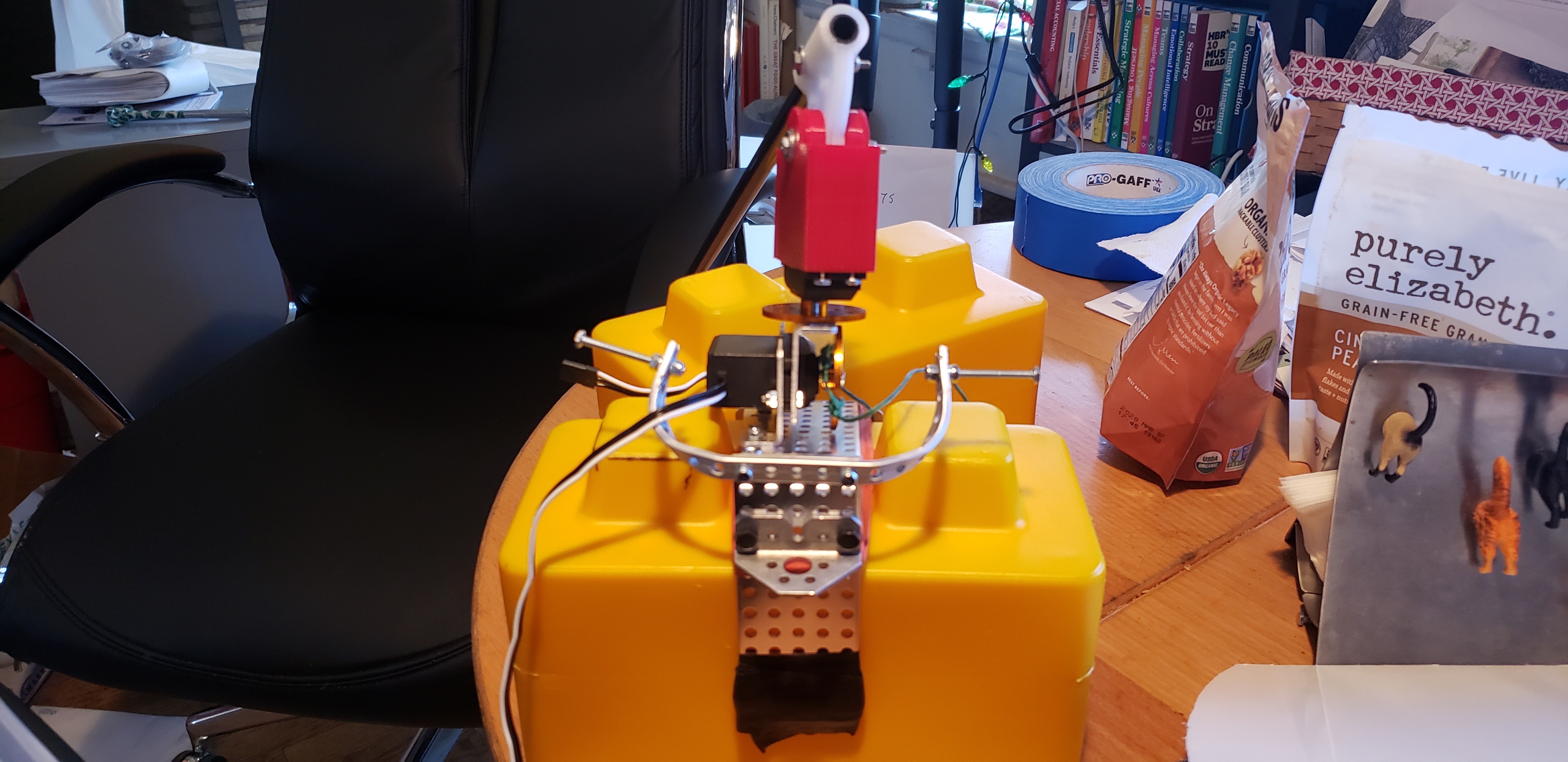
 We also designed and printed square pieces to go on the top and bottom of the gripper to keep it in place.


 This design was too rigid, we overlooked the fact that triangles tend to be the strongest shape, and therefore this octopucker wasn't as compliant as we wanted, damaging the blocks.
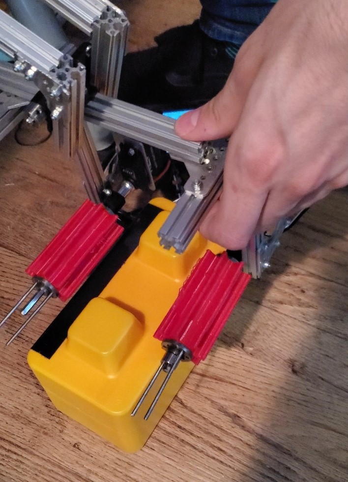
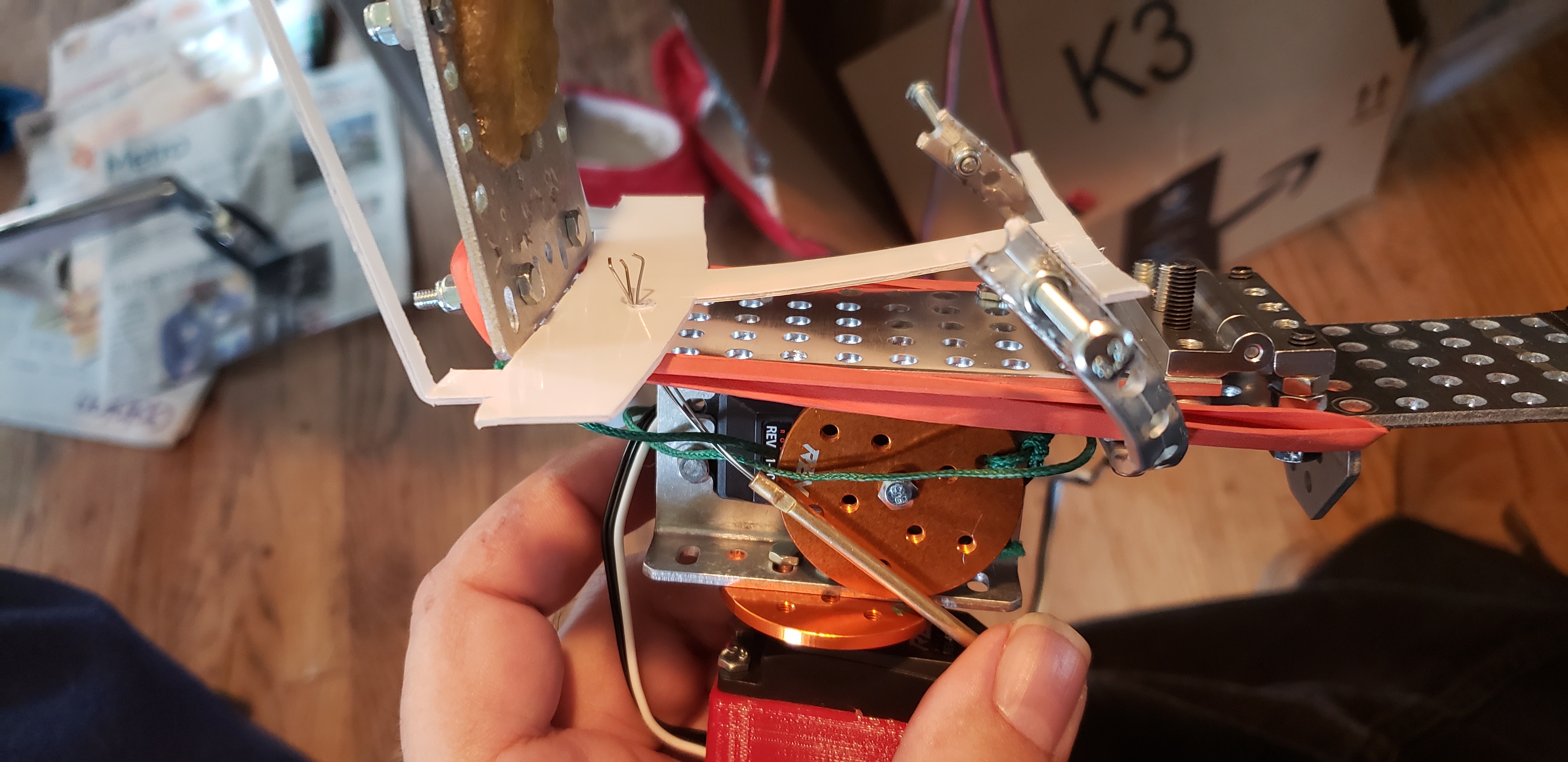
 This design was really good, and we used it for 3-4 tournaments. Our initial design of these wouldn't damage the blocks significantly at the levels we used, but at extraordinary conditions they would gouge the blocks, and under normal conditions they would leave superficial scratches.
 This design was really bad. They would catch on each other and get stuck on themselves, and as a result wouldn't pick up blocks. However, they did not damage the blocks in any conditions. We never brought these to tournament.
 This was a step in the right direction. They didn't grip the blocks that well, but they worked and didn't get stuck on each other or jam.
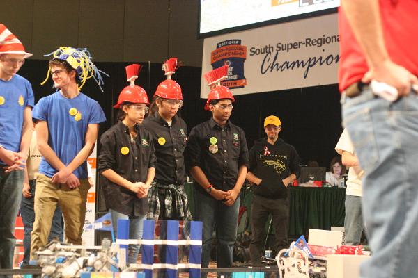
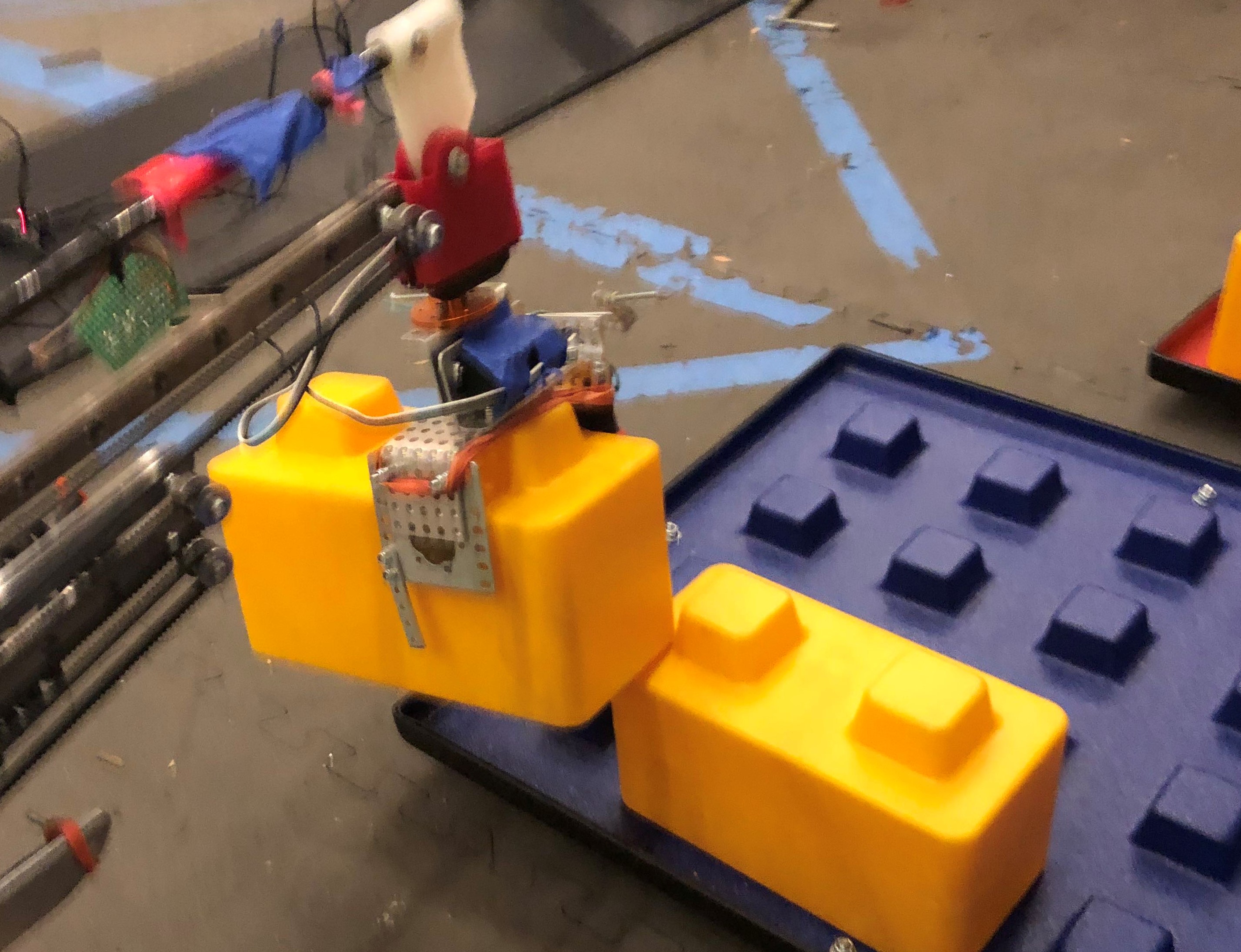
 This is the design we're currently using. It's impossible to damage the blocks with them, and with the slightly larger cylinders, they grip the block really well. We're going to use these going into the South Super Regionals.


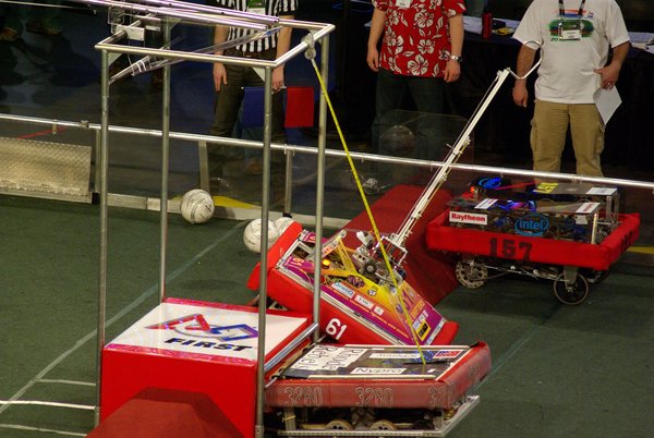
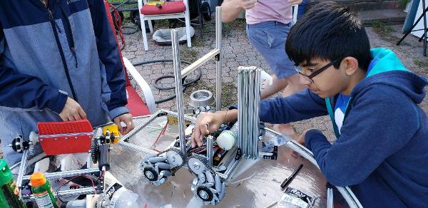
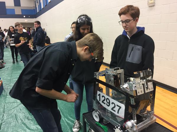
 Austin Lui of Technicbots gets their chassis ready for testing.
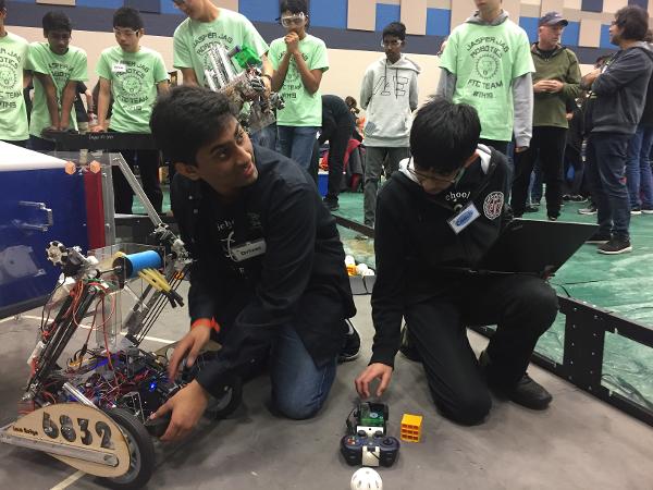
 Connor Mihelic of EFFoRT adds some finishing touches.


 This suggestion uses a plastic flap to "trap" game elements inside it, similar to the lid of a soda cup. You can put marbles through the straw-hole, but you can't easily get them back out.
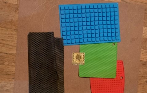
 This one is simple - a linear slide arm attached to a motor so that it can pick up game elements and rotate. We fear, however, that many teams will adopt this strategy, so we probably won't do it. One unique part of our design would be the silicone grips, so that the "claws" can firmly grasp the silver and gold.
 When we did Res-Q, we dropped our robot more times than we'd like to admit. To prevent that, we're designing an interlocking mechanism that the robot can use to hang. It'll have an indent and a corresponding recess that resists lateral force by nature of the indent, but can be opened easily.


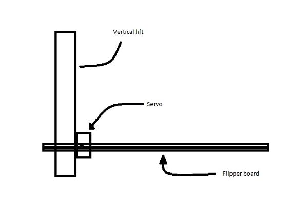
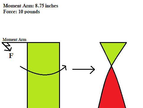
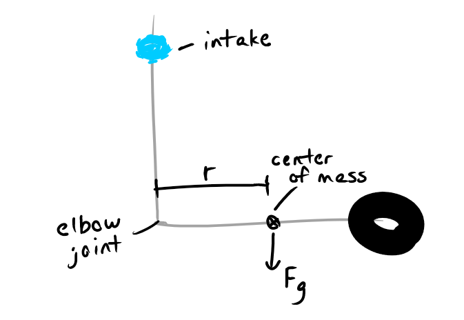
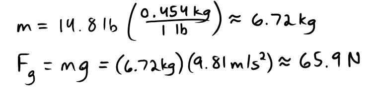
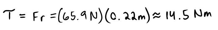
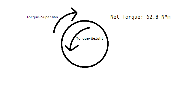
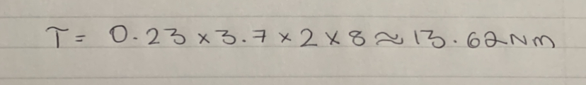
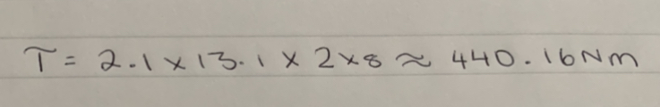
 Then we realized a more pressing issue. Since torque is equal to force * arm length (T=FR), and the force on our robot is only the force due to gravity (F=mg), we had a torque on the lift equal to T=mgR. Then, as the lift was mounted at the very end, the torque on the arm was at its absolute maximum. And, while we're confident in our building ability, we're not that confident. So, we realized that we'd have to move the lift closer to the middle to minimize torque.


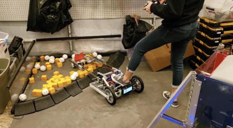


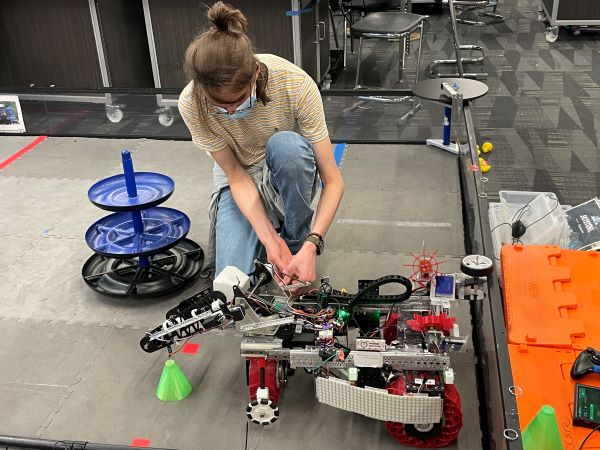
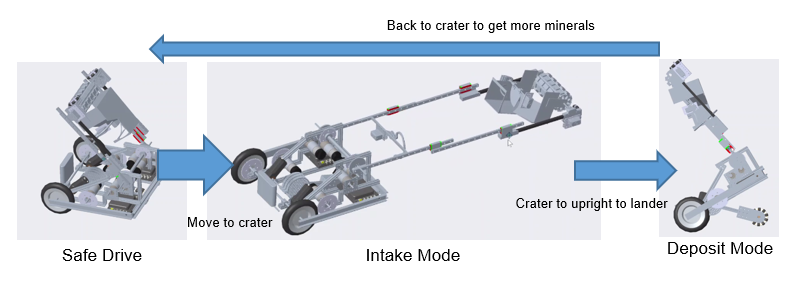
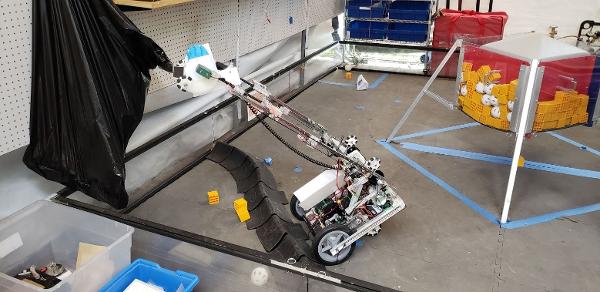
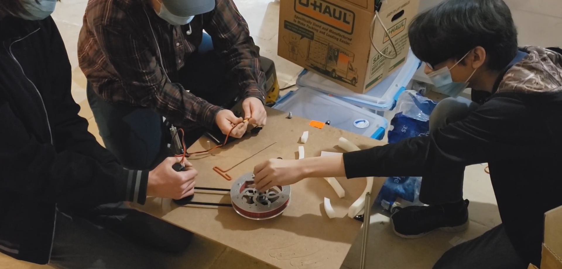
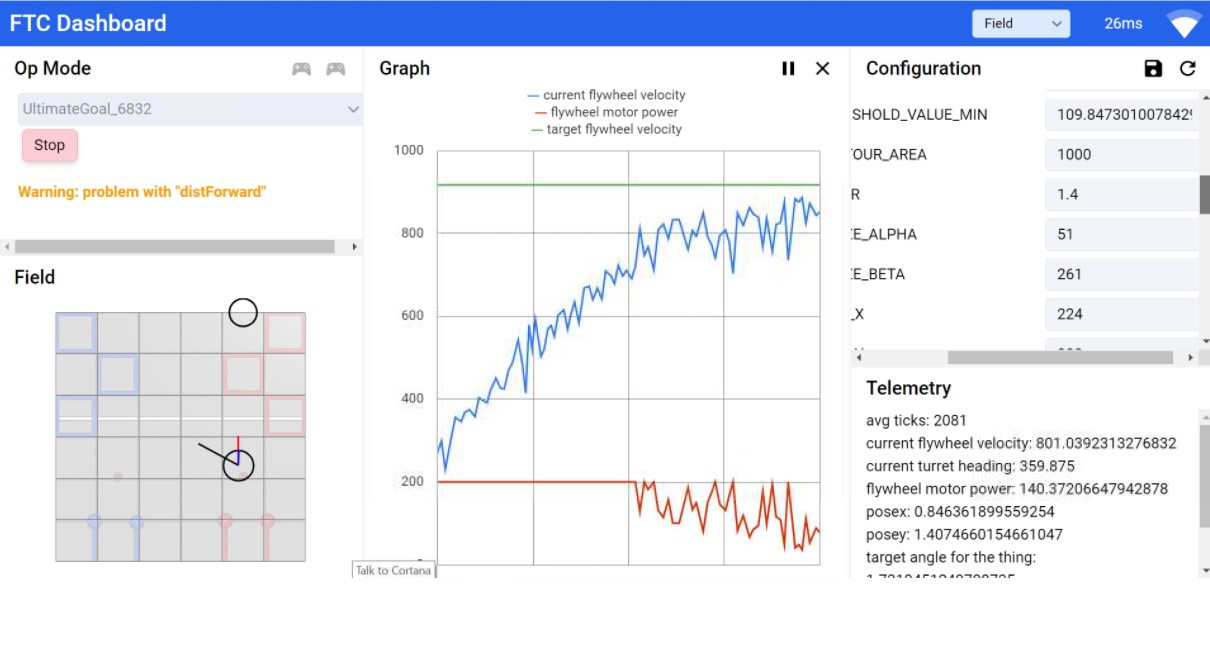
 Karina, Justin, and Jose practiced driving the robot. We discovered that the robot latches extremely well with the new hook and that the autonomous delatch works. We also tested the articulation, or poses, of our robot. The only issue that popped up was when the robot moves into deposit mode, it tips toward the side with linear slides, but Karina discovered that if she drives the robot forward at the same time, she can ram the robot into the correct position. Karina got to 4-5 cycles per match with the new updates. This practice was a way to test the strength of our robt - we've had our robot break under stressful situations previously - and this time nothing broke. The biggest issue was that a servo wire on our intake came unplugged, but even with that, our robot still worked.
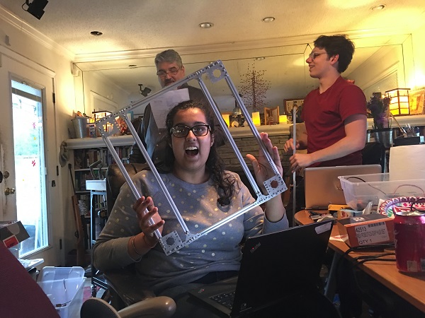
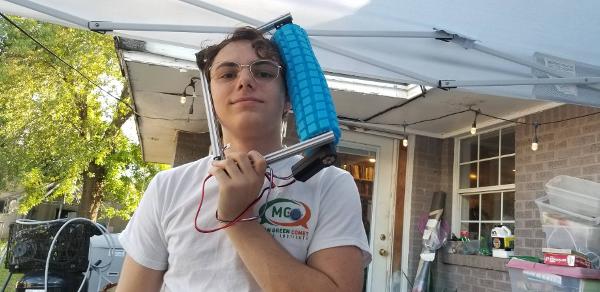
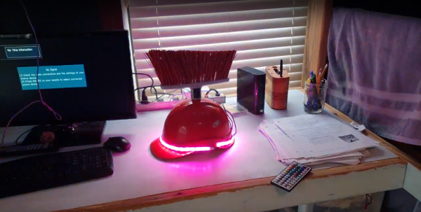 We finished the light-up LED hat.
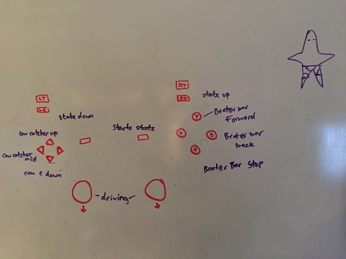
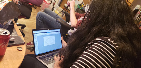 Arjun continued writing the Control Award submission, adding in the new articulations and poses of the driver enhancements. Janavi created state diagrams for the code to add to the submission.


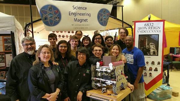
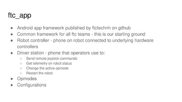
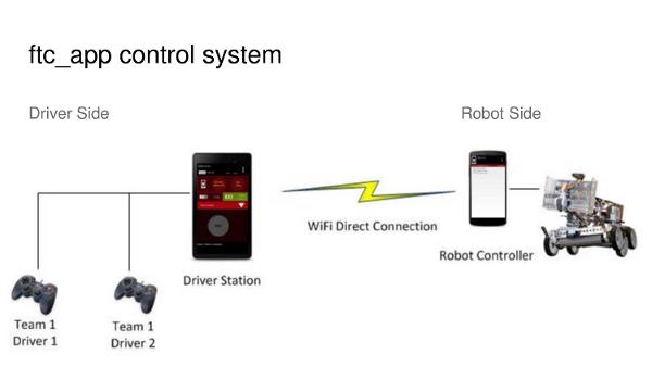
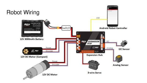
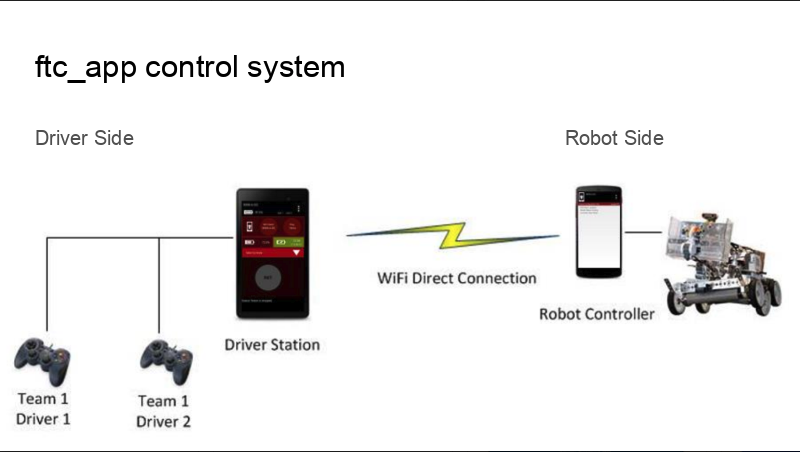
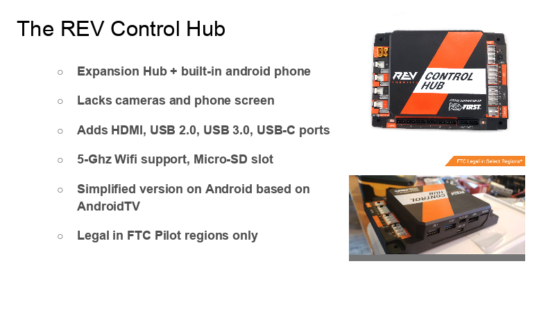
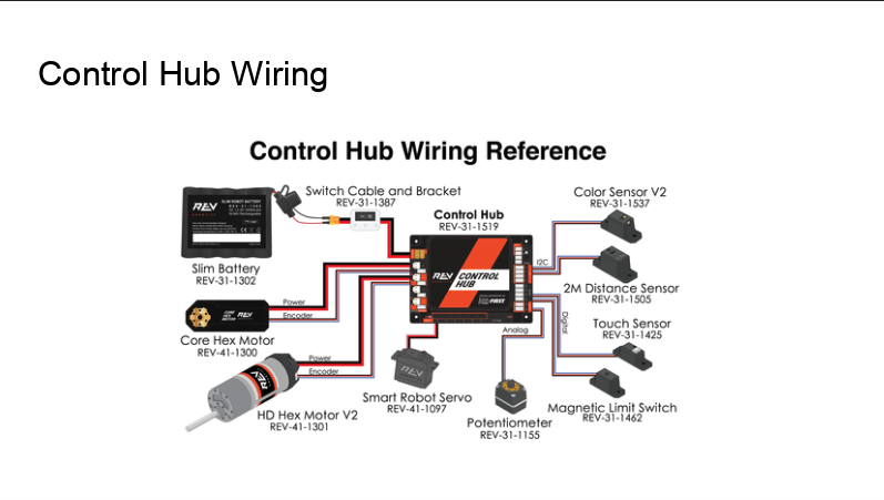
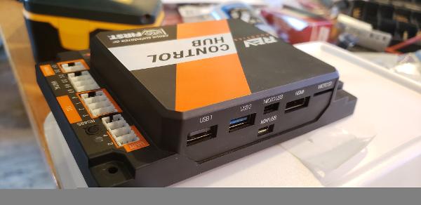 Iron Reign was recently selected to attend a REV Control Hub trial along with select other teams in the region. We wanted to do this so that we could get a good look at the control system that FTC would likely be switching to in the near future, as well as get another chance to test our robot in tournament conditions before Worlds.
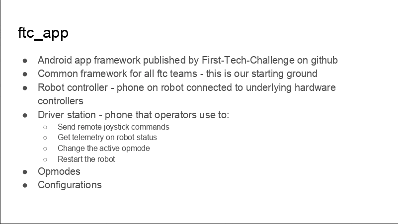
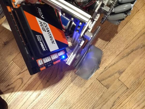 While testing it, we didn't have time to copy over our entire codebase, so we made a quick OpMode that moved one wheel of one of our old robots. Because the provided SDK is almost identical to ftc_app, no changes were needed to the existing sample OpModes. We successfully tested our OpMode, proving that it works fine with the new system.


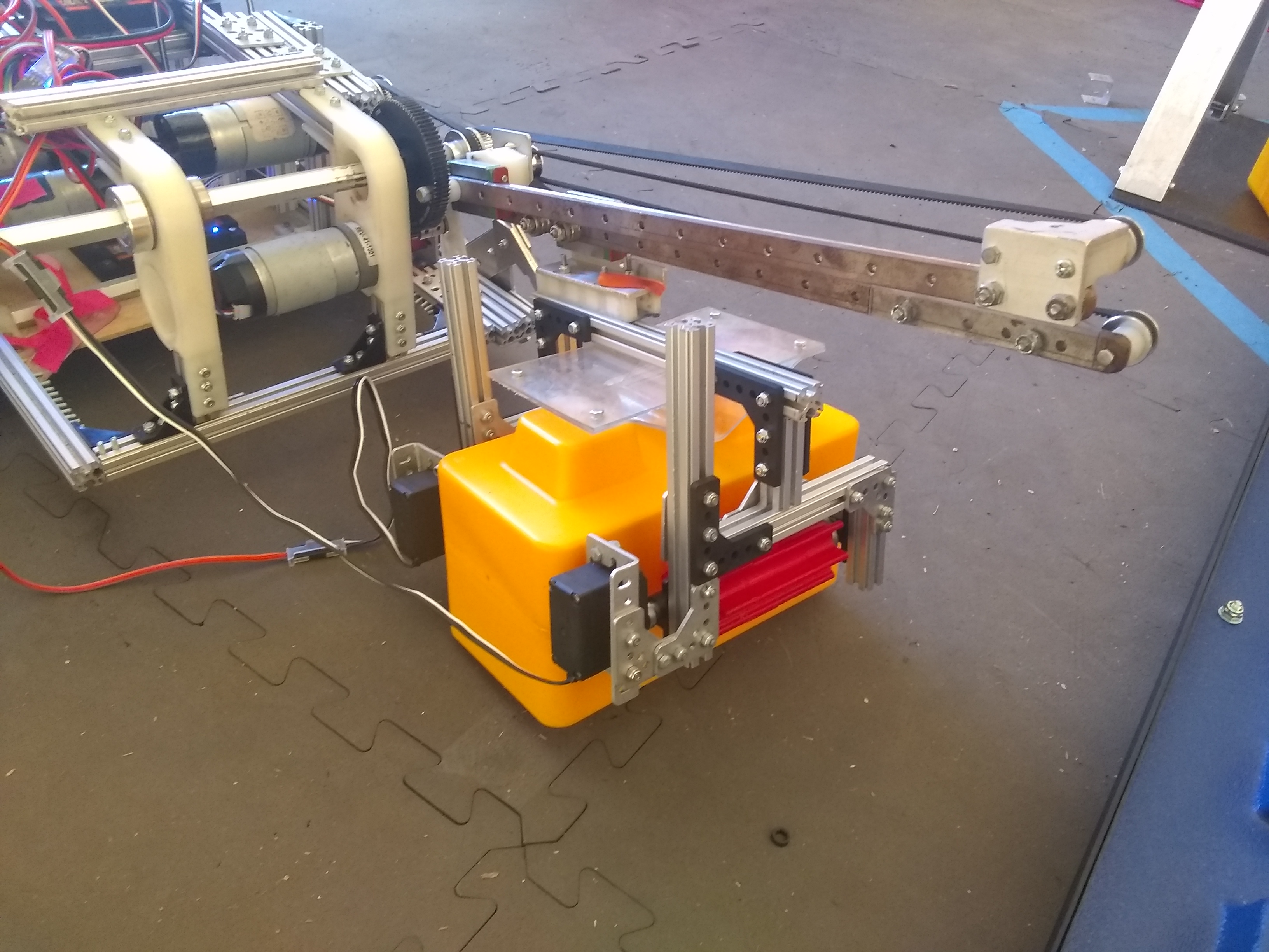

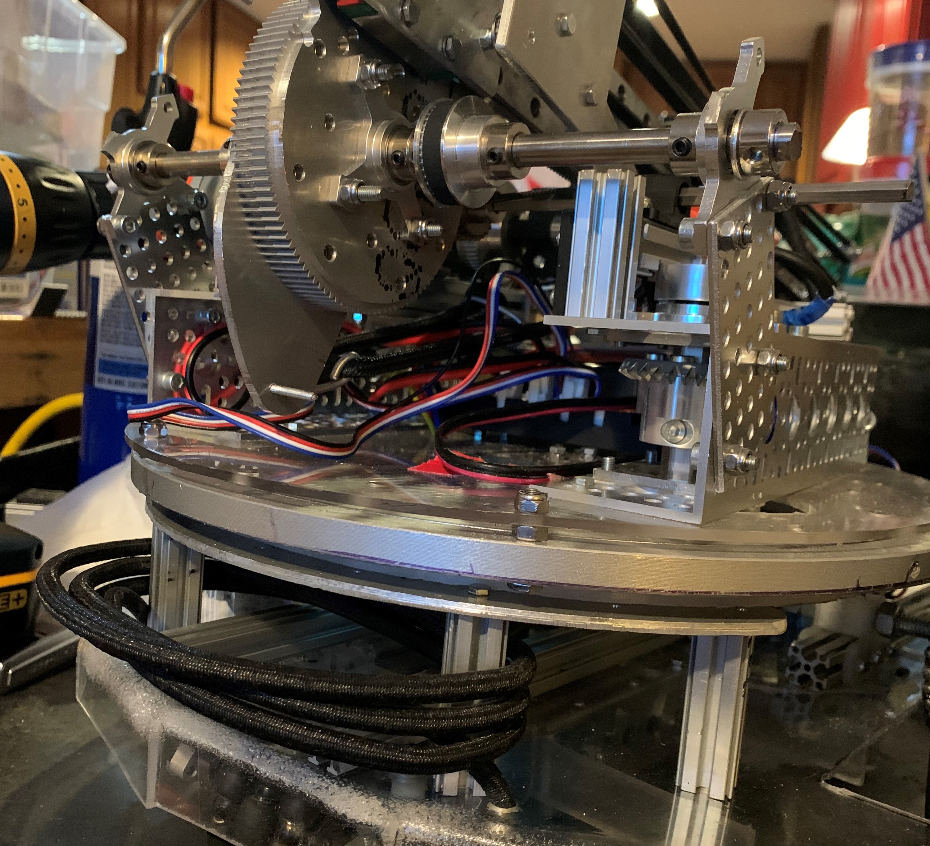
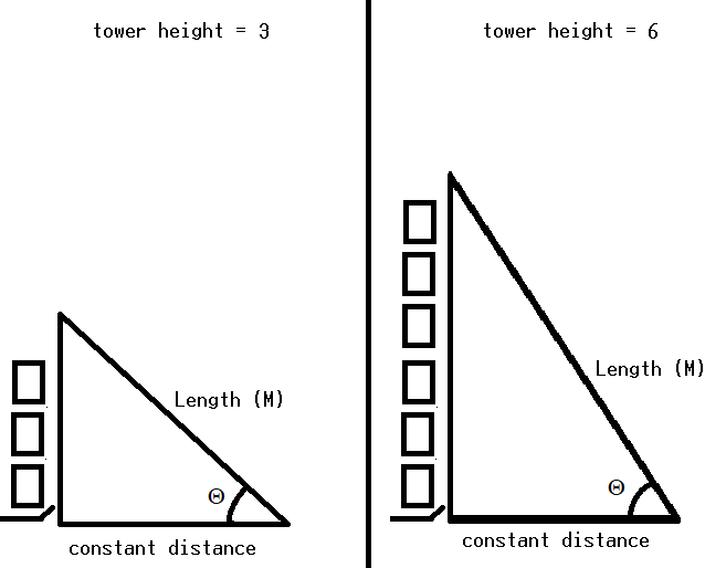
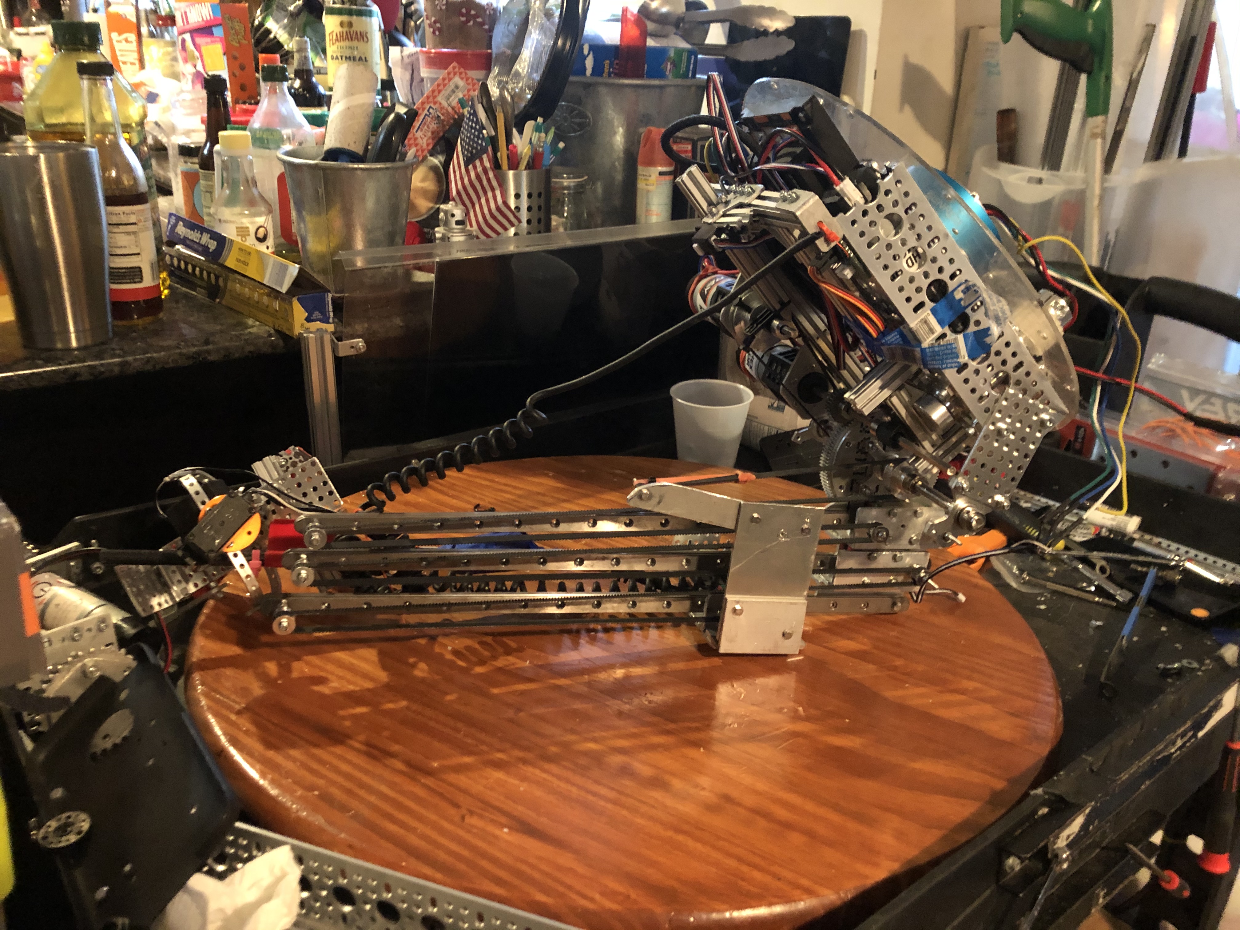


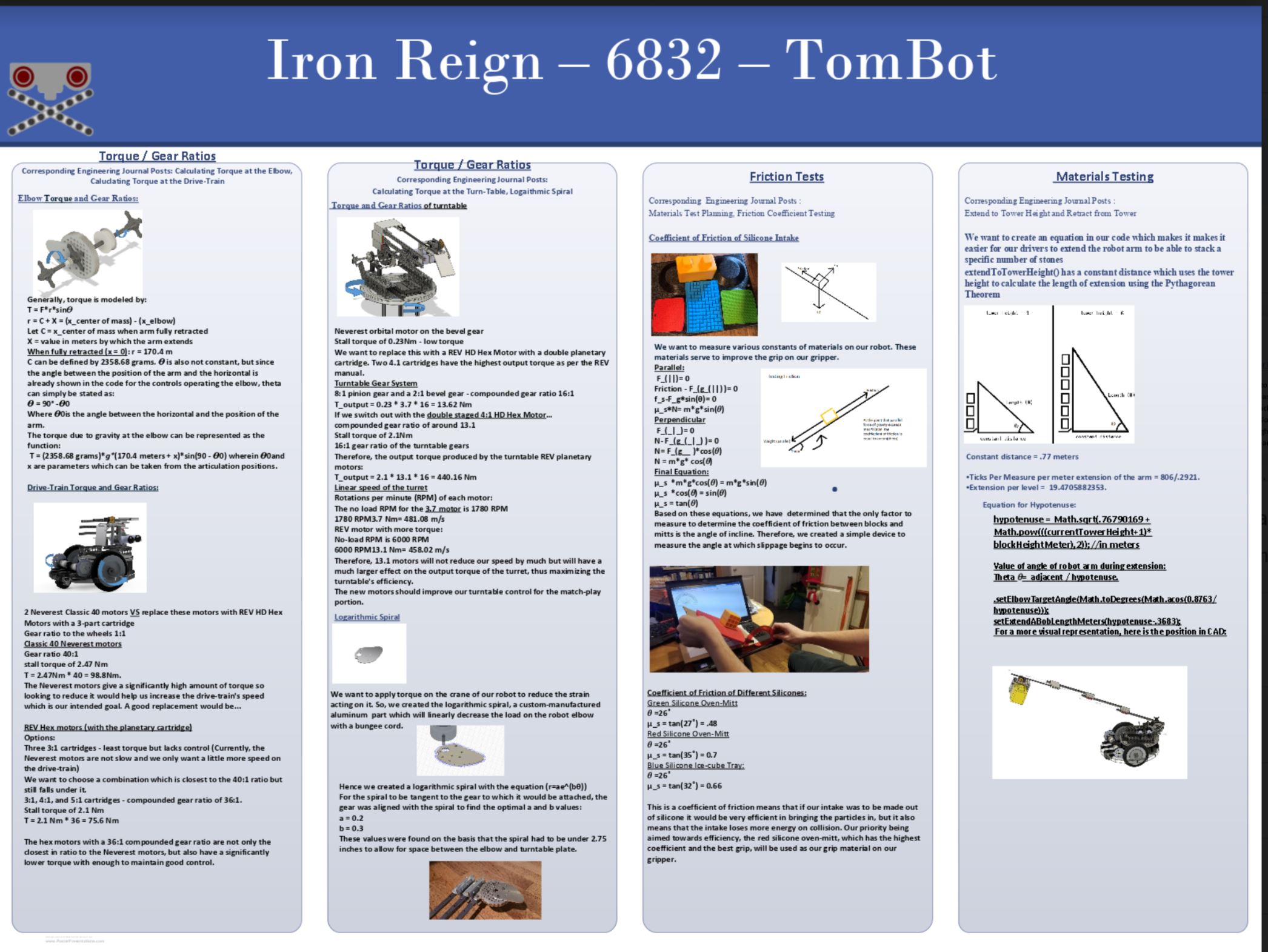


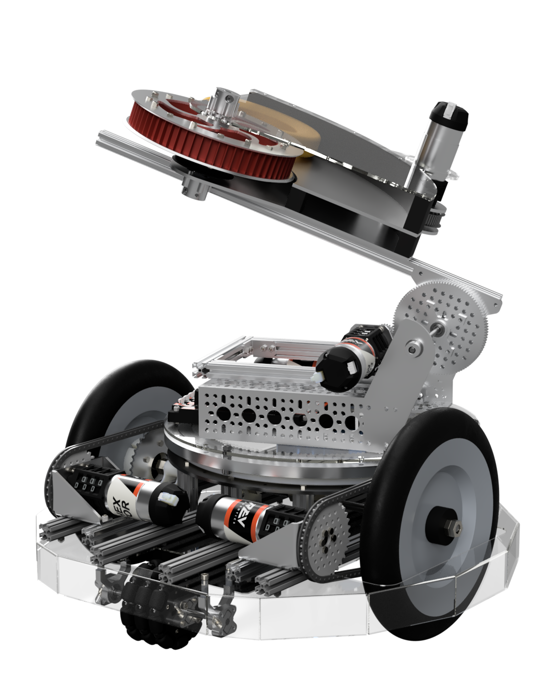
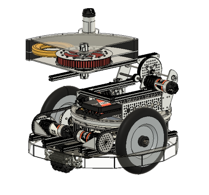


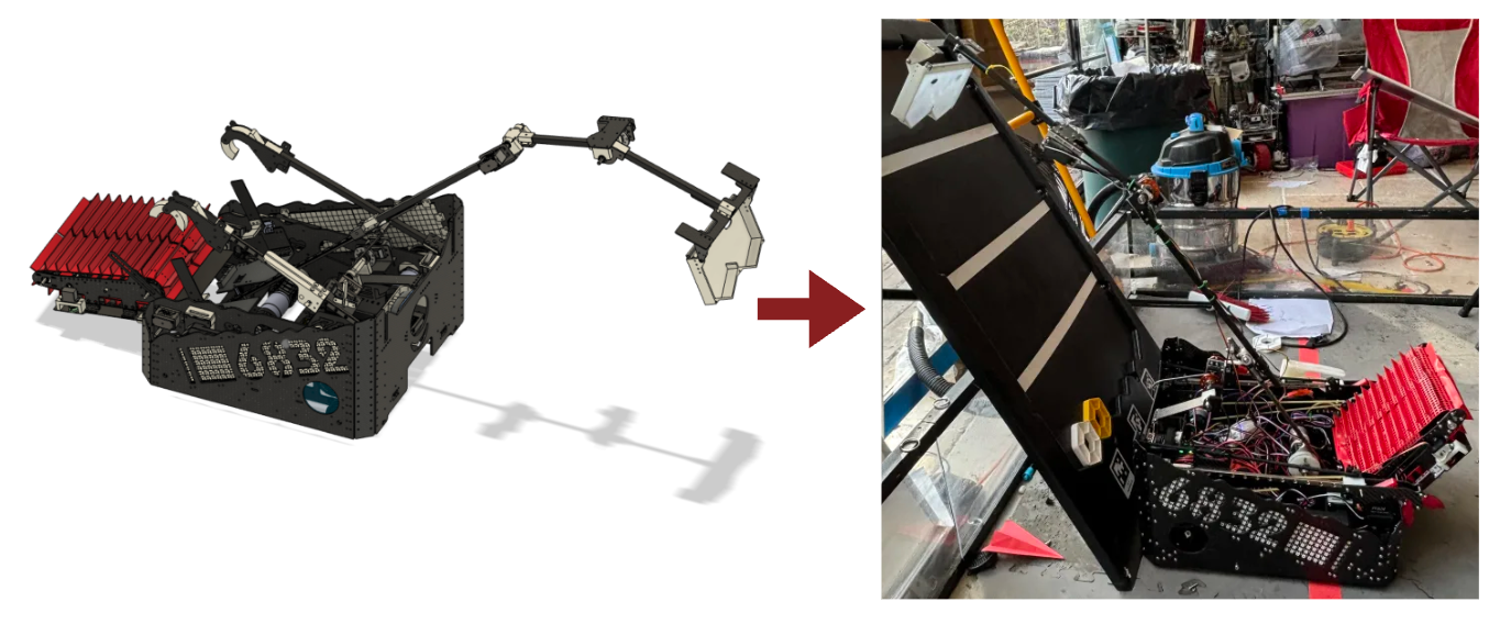
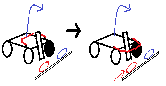
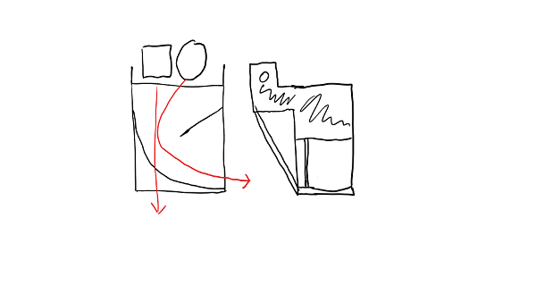
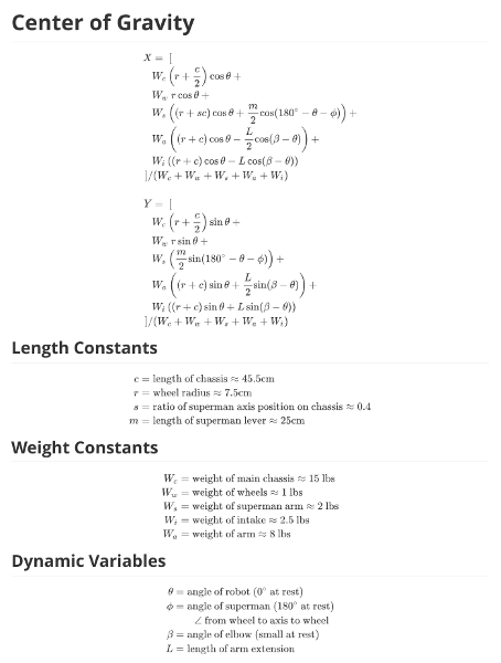
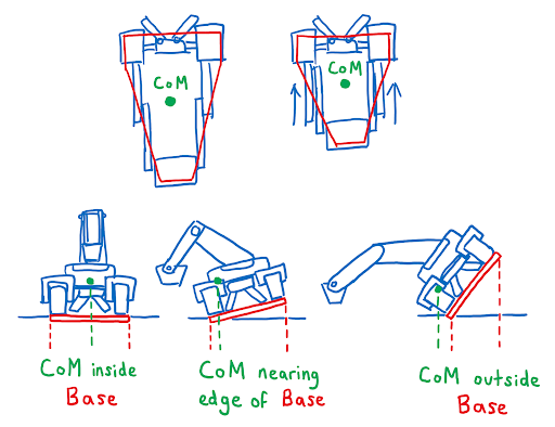 Looking at these diagrams of the robot and its center of mass, we can see how as the crane extends past the base of the robot, the center of mass moves towards the base. Eventually, the center of mass reaches a position outside of the base and the robot falls over. To solve this problem, we would have to either lower the center of mass or limit its fluctuation during movement.
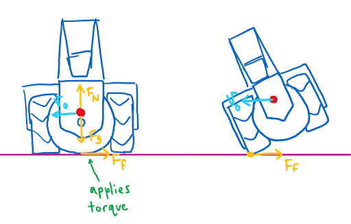
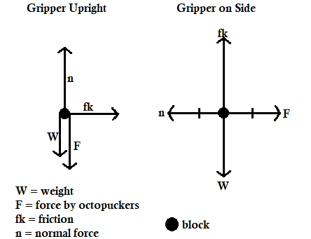
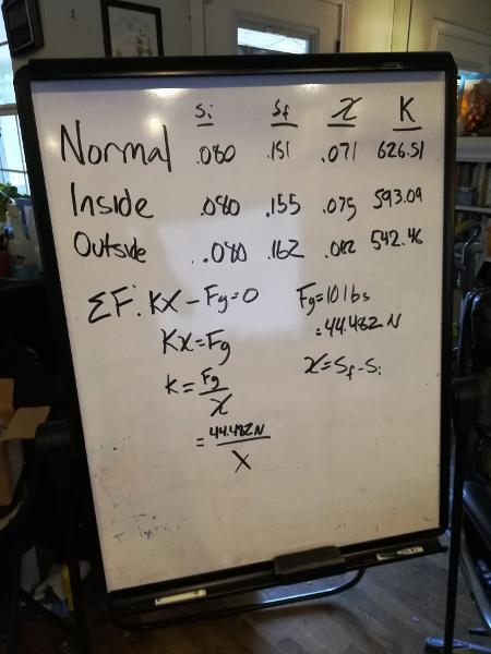
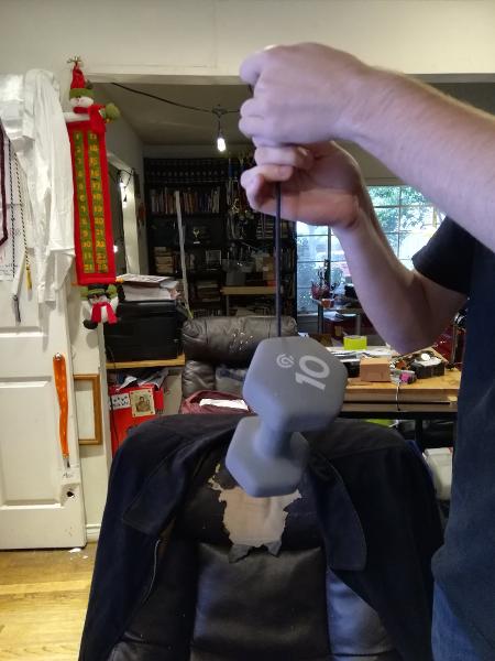
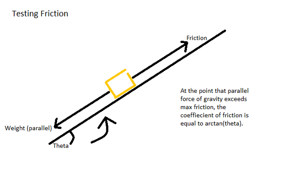
 You can see from these free-body diagrams that as we lower the vertical component of the normal force, the overall rotational torque exerted by the swerve module is decreased, which inspired our decisions to lower the center of mass.
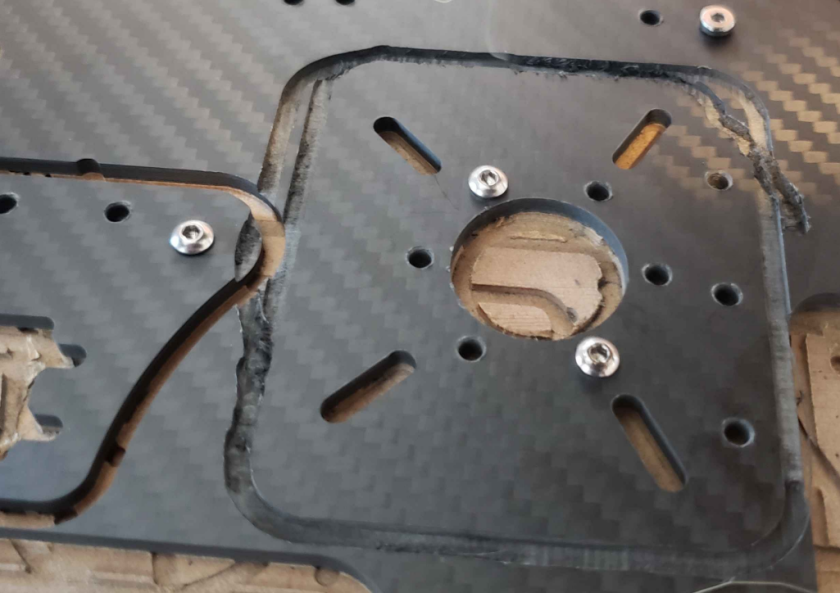
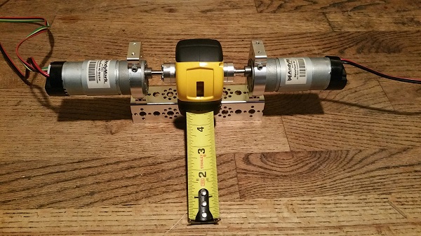
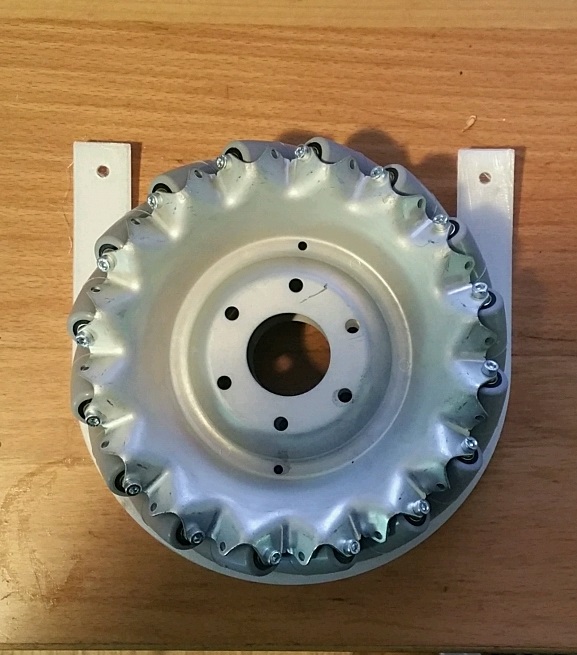
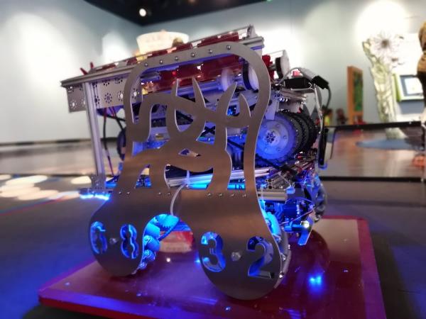
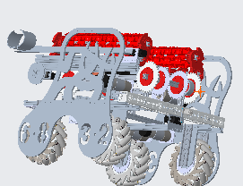
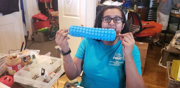
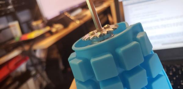
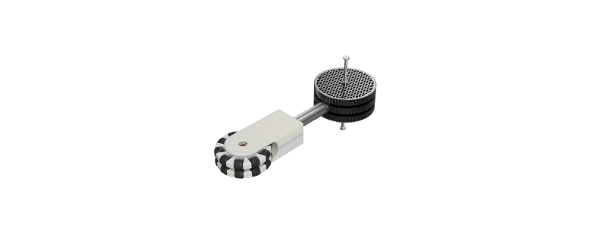
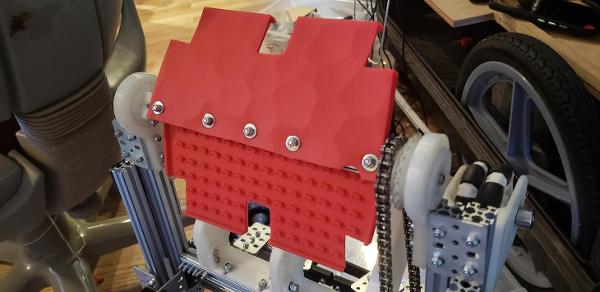
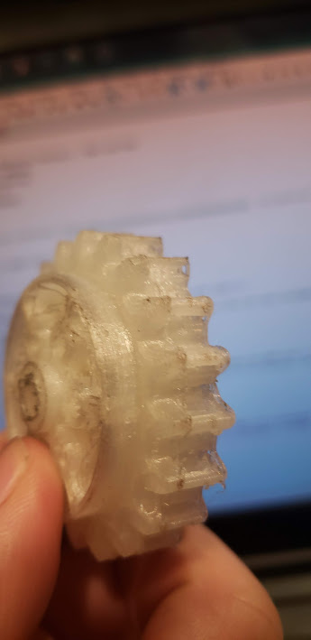
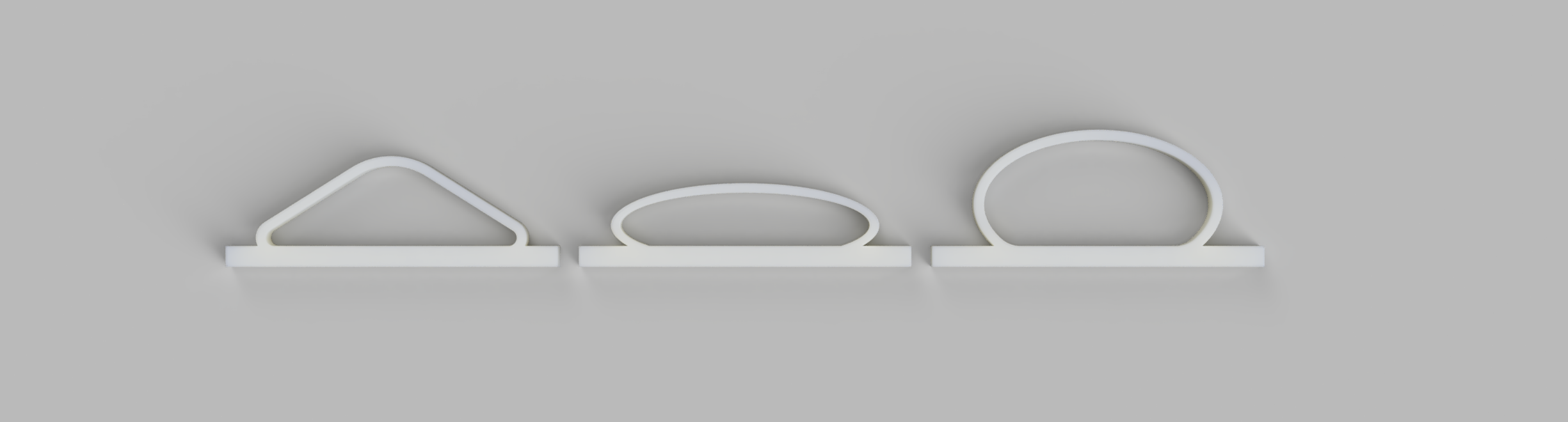
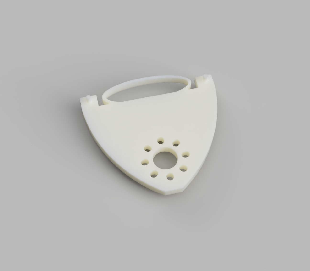
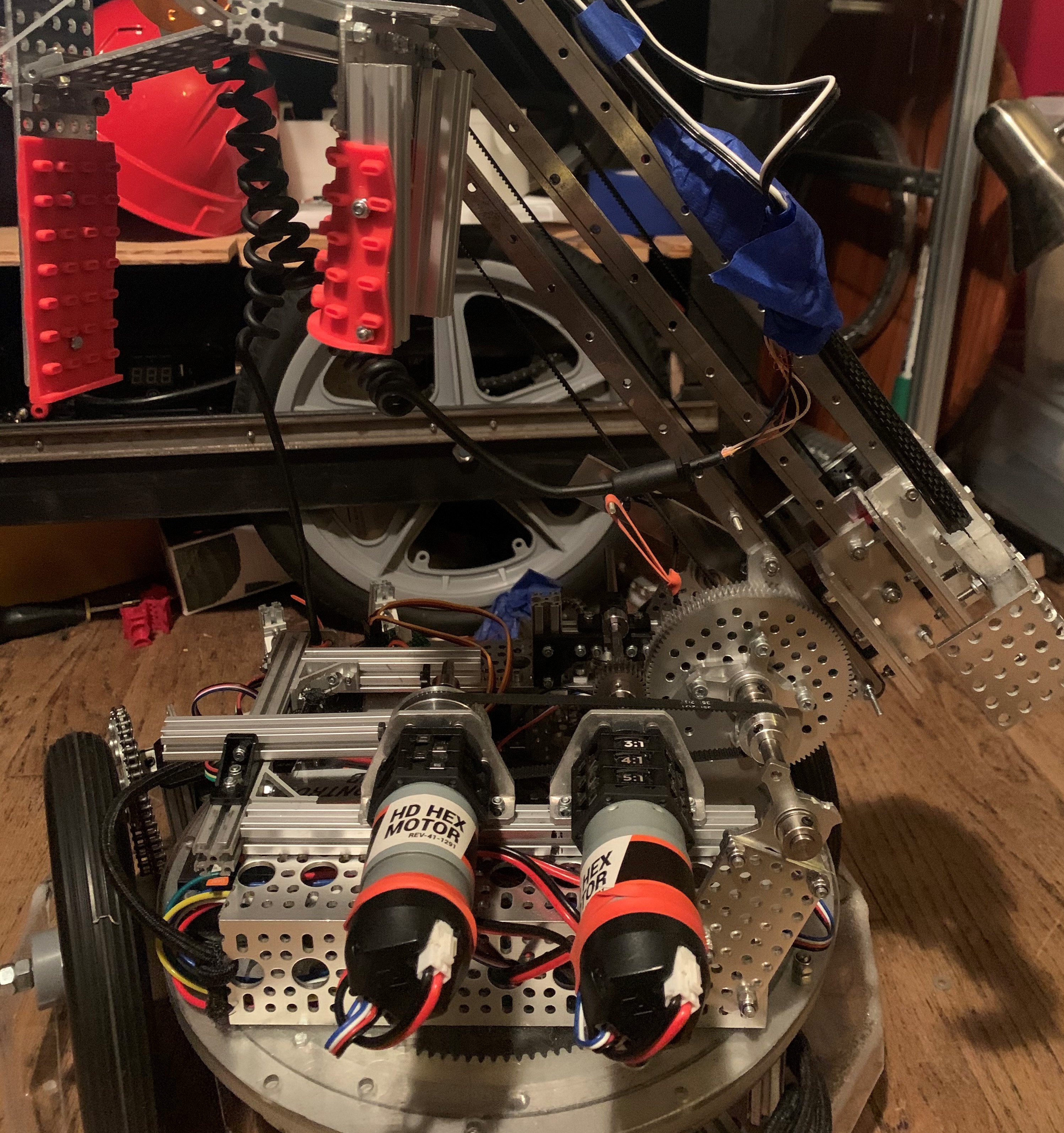
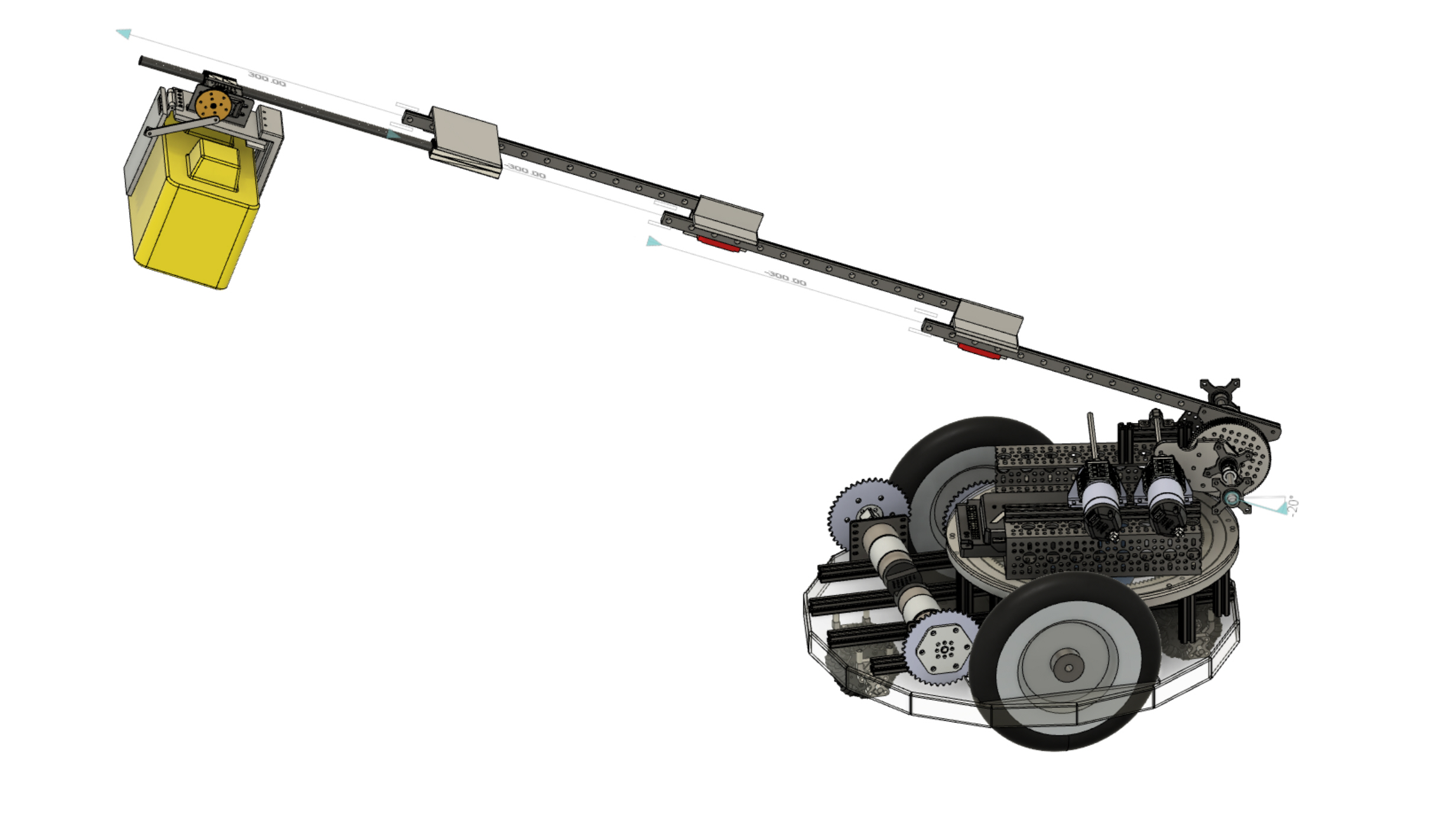
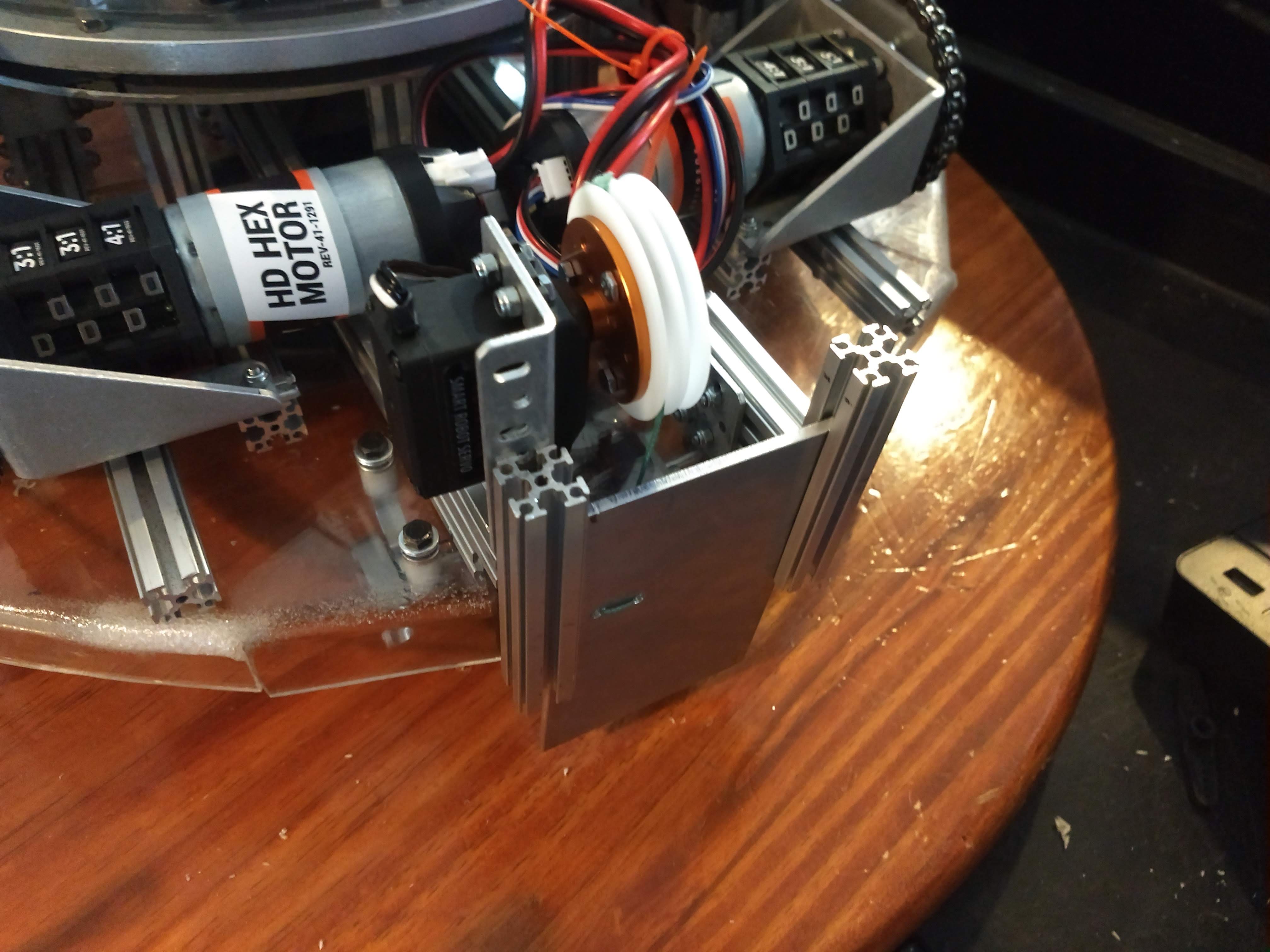
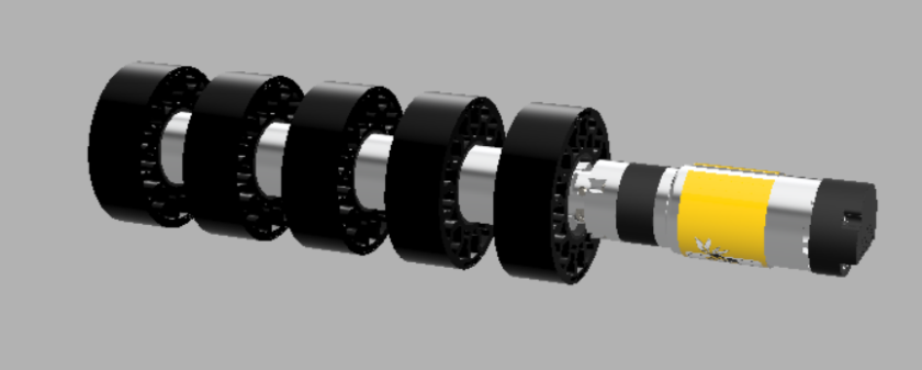
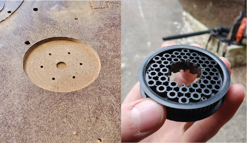
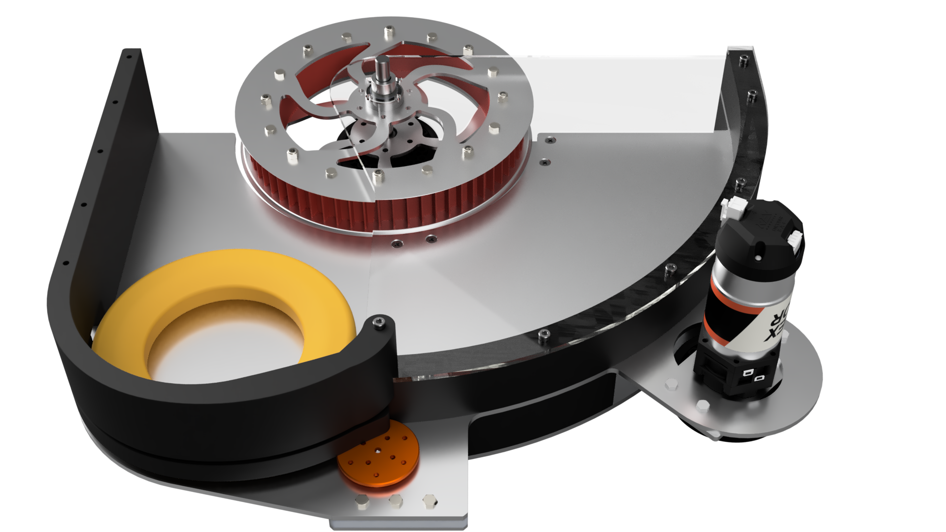
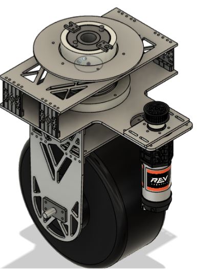
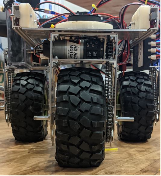
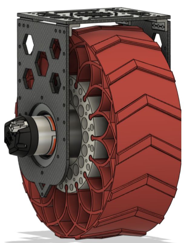
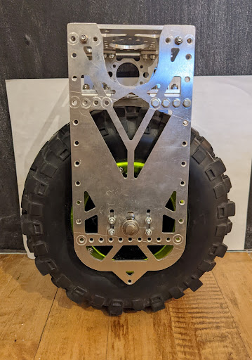
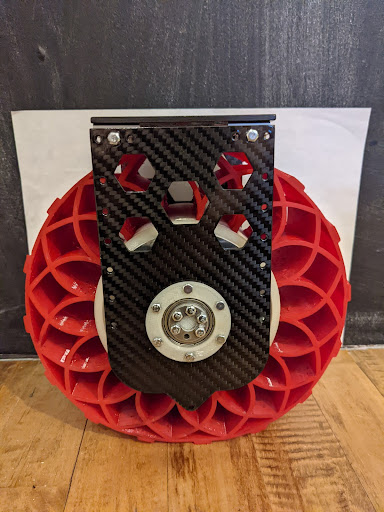
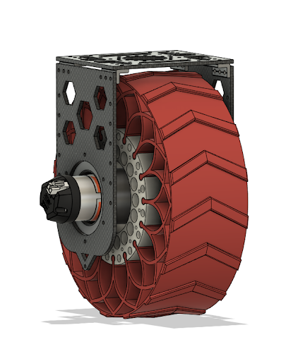
We did this by redesigning our wheel modules and moving the motor further down. Our redesigned wheel modules utilize custom printed "barrier beaters" instead of the rock climbers we used before. These wheels were printed out of ninja flex and nylon and utilized a Gothic Arch design inspired by Monash University's rover wheels. The custom wheel modules used custom carbon-fiber plates and holes in the nylon hub to help reduce weight. Overall, these wheels were excellent at traversing the barriers, weighed less, and the wheel module allowed the motor to drop 5 inches in height. This led to a lower center of mass for the robot.
You can see from these free-body diagrams that as we lower the vertical component of the normal force, the overall rotational torque exerted by the swerve module is decreased, which inspired our decisions to lower the center of mass.
We did this by redesigning our wheel modules and moving the motor further down. Our redesigned wheel modules utilize custom printed "barrier beaters" instead of the rock climbers we used before. These wheels were printed out of ninja flex and nylon and utilized a Gothic Arch design inspired by Monash University's rover wheels. The custom wheel modules used custom carbon-fiber plates and holes in the nylon hub to help reduce weight. Overall, these wheels were excellent at traversing the barriers, weighed less, and the wheel module allowed the motor to drop 5 inches in height. This led to a lower center of mass for the robot.
 However, in the situation that the crane and robot extension did lead to the center of mass nearing the base, we installed an outrigger system as a preventative measure. An outrigger is essentially a beam that extends from a robot that is used to improve stability. Our outriggers used omni wheels and functioned similarly to training wheels, preventing the robot from tipping over when the crane moves out and extends.
 Finally, we implemented some code changes to help deal with this problem, building anti-tipping limiters which allowed for gradual acceleration. This prevented the sudden acceleration mentioned earlier which was a cause of our tipping issue. We also programmed in pre-set arm locations to help keep the center of mass near the wheelbase, making sure that the center of mass never passes the base of the actual robot.